plot
- postprocessinglib.evaluation.visuals.plot(merged_df: DataFrame = None, df: DataFrame = None, sim_df: DataFrame = None, step: bool = False, where: str = 'pre', legend: tuple[str, str] = ('Data',), metrices: list[str] = None, metric_options: dict | None = None, components: tuple[str, ...] | None = None, mode: str = 'median', models: List[str] = None, grid: bool = False, minor_grid: bool = False, title: str = None, labels: list[str] = None, padding: bool = False, linestyles: tuple[str, str] = ('r-',), linewidth: tuple[float, float] = (1.5,), fig_size: tuple[float, float] = (10, 6), font_size: int = 12, text_size: int = 12, metrics_adjust: tuple[float, float] = (1.05, 0.5), plot_adjust: float = 0.2, save: bool = False, save_as: str = None, dir: str = '/home/docs/checkouts/readthedocs.org/user_builds/nhs-postprocessing/checkouts/latest/docs/source') figure
Create a comparison time series line plot of simulated and optionally, observed time series data
This function generates line plots for any number of simulated and optionally observed data
The function can handle data provided in three formats: - A merged DataFrame containing both observed and simulated data. - A Single DataFrame of your choosing. - A DataFrame containing only simulated data.
The plot allows customization of various visual elements like line style, colors, axis labels, and title. The resulting figure can be displayed or saved to a specified directory and file name.
- Parameters:
merged_df (pd.DataFrame, optional) – The dataframe containing the series of observed and simulated values. It must have a datetime index. To be use when the data contains both observed and simulated values.
sim_df (pd.DataFrame, optional) – A DataFrame containing only the simulated data series
df (pd.DataFrame, optional) – A Single DataFrame usually containing only one of either simulated or observed data… or any data.
step (bool, optional) – Whether to plot the data as a step plot. Default is False, which plots a regular line plot.
where (str, optional) – The location of the step in the step plot. Default is ‘pre’, which means the step occurs before the x value.
legend (tuple of str, optional) – A tuple containing the labels for the data being plotted
metrices (list of str, optional) – A list of metrics to display on the plot, default is None.
grid (bool, optional) – Whether to display a grid on the plot, default is False.
minor_grid (bool, optional) – Whether to display a minor grid on the plot, default is False.
title (str, optional) – The title of the plot.
labels (list of strs, optional) – A tuple containing the labels for the x and y axes.
padding (bool, optional) – Whether to add padding to the x-axis limits for a tighter plot, default is False.
linestyles (tuple of str, optional) – A tuple specifying the line styles for the simulated and observed data.
linewidth (tuple of float, optional) – A tuple specifying the line widths for the simulated and observed data.
fig_size (tuple of float, optional) – A tuple specifying the size of the figure.
font_size (int, optional) – The font size for the plot text, default is 12.
text_size (int, optional) – The font size for the metrics text on the plot, default is 12.
metrics_adjust (tuple of float, optional) – A tuple specifying the position for the metrics on the plot.
plot_adjust (float, optional) – A value to adjust the plot layout to avoid clipping.
mode (str, optional) – The mode used to calculate the metric for the scatter plot. Default is ‘median’. But it can be ‘models’ or ‘mean’. It can also be models used to indicate that the metric is to be calculated for each model as specified in the models list.
models (list of str, optional) – A list of model names to be used when calculating the metric for the scatter plot. Default is None. It is only used when mode is ‘models’.
save (bool, optional) – Whether to save the plot to a file, default is False.
save_as (str or list of str, optional) – The name or list of names to save the plot as. If a list is provided, each plot will be saved with the corresponding name.
dir (str, optional) – The directory to save the plot to, default is the current working directory.
- Returns:
fig
- Return type:
Matplotlib figure instance and/or png files of the figures.
Examples
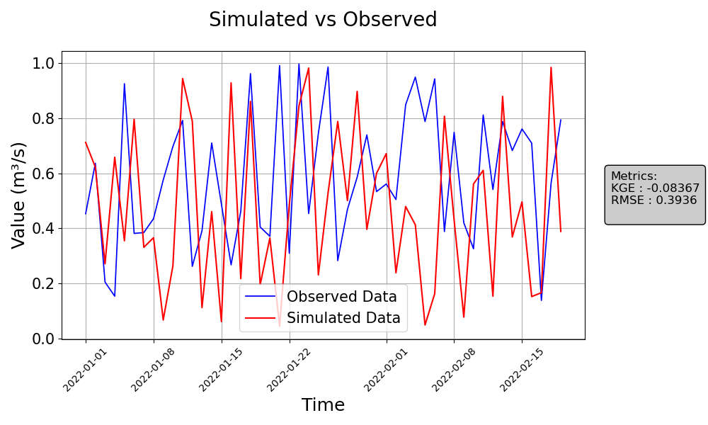
>>> from postprocessinglib.evaluation import visuals
>>> # Example 1: Plotting merged data with simulated and observed values
>>> merged_data = pd.DataFrame({...})  # Your merged dataframe
>>> visuals.plot(merged_df = merged_data,
                title='Simulated vs Observed',
                labels=['Time', 'Value'], grid=True,
                metrices = ['KGE','RMSE'])
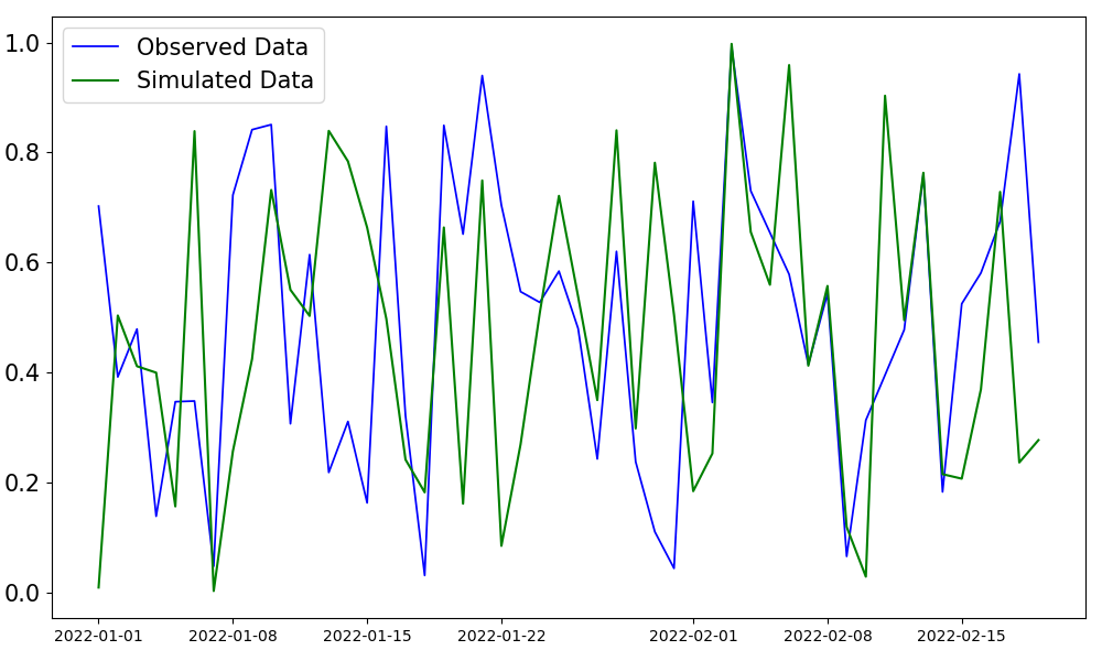
>>> # Example 2: Plotting only observed and simulated data with custom linestyles and saving the plot
>>> obs_data = pd.DataFrame({...})  # Your observed data
>>> sim_data = pd.DataFrame({...})  # Your simulated data
>>> visuals.plot(obs_df = obs_data, sim_df = sim_data, linestyles=('g-', 'b-'),
                save=True, save_as="plot2_example", dir="../Figures")
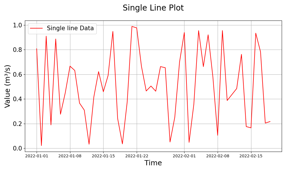
>>> # Example 3: Plotting a single dataframe
>>> single_data = pd.DataFrame({...})  # Your single dataframe (either simulated or observed)
>>> visuals.plot(df=single_data, grid=True, title="Single Line Plot", labels=("Time", "Value"))
Notes
The function requires at least one valid data input (merged_df, sim_df, or df).
The time index of the input DataFrames must be a datetime index or convertible to datetime.
If the number of columns in the obs_df or sim_df exceeds five, the plot will be automatically saved.
Metrics will be displayed on the plot if specified in the metrices parameter.