Visualizations Tutorial
This notebook provides examples on how to carry out data visualization using the post_processing python library. Be sure to go through the Quick Start section of the documentation for instructions on how to access and import the libary and its packages.
If you would like to open an editable runnable version of the tutorial click here to be directed to a binder platform
The Library is still under active development and empty sections will be completed in Due time
Table of content
All files are available in the github repository here
Requirements
The conda environmnent contains all libraries associated the post processing library. After setting up the conda environment, you only have to import the visualization modules from postprocessinglib.evaluation.
In this example though, I will also be importing other modules to help generate the data that I will be trying to visualize.
[2]:
import pandas as pd
from postprocessinglib.evaluation import data, visuals
Lets use one of the data blocks from the data manipulation tutorial
Now that we have our data, let’s jump right in!
[3]:
# passing a controlled csv file for testing
path_output = "MESH_output_streamflow_3.csv"
path_input = "Station_data.xlsx"

DATAFRAMES = data.generate_dataframes(csv_fpaths=path_output, warm_up=365,
                                      daily_agg = True, da_method = 'min',
                                      weekly_agg = True, wa_method = 'min',
                                      monthly_agg = True, ma_method = 'inst',
                                      yearly_agg = True, ya_method = 'sum',
                                      seasonal_p = True, sp_dperiod = ('04-01', '08-30'), sp_subset = ('1981-01-01', '1985-12-31'),
                                      long_term = True, lt_method = ["mean" ,'q75' ,'Q25', 'q10', 'q90'],
                                      stat_agg = True, stat_method = ['sum', 'sum', 'min'],)
Stations = pd.read_excel(io=path_input)

ignore = []
for i in range(0, len(Stations)):
    if Stations['Properties'][i] == 'X':
        ignore.append(i)

Stations = Stations.drop(Stations[Stations['Properties'] == 'X'].index)
Stations = Stations.set_index('Station Number')

for i in reversed(ignore):
        DATAFRAMES["DF_OBSERVED"] = DATAFRAMES["DF_OBSERVED"].drop(columns = DATAFRAMES['DF_OBSERVED'].columns[i])
        DATAFRAMES['DF_SIMULATED']  = DATAFRAMES["DF_SIMULATED"].drop(columns = DATAFRAMES['DF_SIMULATED'].columns[i])
        for key, dataframe in DATAFRAMES.items():
            if key == "DF_1" or key == "DF_2" or key == "DF":
                DATAFRAMES[key] = dataframe.drop(columns = dataframe.columns[[2*i, 2*i+1]])
            if key == "DF_MERGED":
                DATAFRAMES[key] = dataframe.drop(columns = dataframe.columns[[2*i, 2*i+1, 2*i+2]])


for key, value in DATAFRAMES.items():
    print(f"{key}:\n{value.head}")
The start date for the Data is 1982-10-02
DF:
<bound method NDFrame.head of QOMEAS_05AA024 QOSIM_05AA024 QOMEAS_05AB046 QOSIM_05AB046 \
1982-10-02 15.00 12.727950 NaN 2.151088
1982-10-03 14.80 12.070300 NaN 1.282258
1982-10-04 15.20 11.928440 NaN 0.864993
1982-10-05 15.00 11.873910 NaN 0.662052
1982-10-06 14.10 11.845160 NaN 0.560041
... ... ... ... ...
2016-12-27 8.62 0.626161 NaN 0.426263
2016-12-28 8.64 0.619734 NaN 0.425050
2016-12-29 8.63 0.612944 NaN 0.423842
2016-12-30 8.64 0.606437 NaN 0.422638
2016-12-31 8.61 0.599758 NaN 0.421438
QOMEAS_05AC003 QOSIM_05AC003 QOMEAS_05AD007 QOSIM_05AD007 \
1982-10-02 1.840 1.452520 37.6 41.470610
1982-10-03 1.840 1.230331 39.6 28.868720
1982-10-04 1.690 1.087916 38.7 23.806940
1982-10-05 1.580 0.993243 37.6 21.888450
1982-10-06 1.430 0.918875 29.8 21.085320
... ... ... ... ...
2016-12-27 0.966 0.341739 20.7 6.993578
2016-12-28 1.010 0.339073 22.0 6.978570
2016-12-29 1.030 0.336443 24.5 6.963836
2016-12-30 1.030 0.333846 25.5 6.949335
2016-12-31 1.010 0.331275 25.1 6.935077
QOMEAS_05AG006 QOSIM_05AG006 ... QOMEAS_05HD039 QOSIM_05HD039 \
1982-10-02 31.2 82.633610 ... 1.48 0.004145
1982-10-03 39.7 72.782590 ... 1.36 0.101997
1982-10-04 41.9 58.236480 ... 1.29 0.120259
1982-10-05 42.2 45.029110 ... 1.31 0.106829
1982-10-06 42.4 35.632970 ... 1.48 0.302513
... ... ... ... ... ...
2016-12-27 21.7 7.146379 ... 1.65 0.113367
2016-12-28 22.6 7.128211 ... 1.67 0.105351
2016-12-29 24.3 7.110573 ... 1.70 0.097989
2016-12-30 25.7 7.093432 ... 1.70 0.091243
2016-12-31 25.8 7.076759 ... 1.71 0.085089
QOMEAS_05HG001 QOSIM_05HG001 QOMEAS_05KD003 QOSIM_05KD003 \
1982-10-02 161.0 211.1882 359.0 378.7940
1982-10-03 162.0 221.3527 209.0 375.5247
1982-10-04 154.0 231.0193 316.0 372.8839
1982-10-05 147.0 231.2442 351.0 371.0161
1982-10-06 169.0 228.5721 319.0 372.7308
... ... ... ... ...
2016-12-27 294.0 223.7898 301.0 347.1989
2016-12-28 291.0 223.8707 424.0 346.5004
2016-12-29 290.0 223.1373 450.0 346.5625
2016-12-30 291.0 223.2267 413.0 345.2052
2016-12-31 296.0 223.6875 415.0 344.2019
QOMEAS_05KE002 QOSIM_05KE002 QOMEAS_05KJ001 QOSIM_05KJ001
1982-10-02 5.49 3.542509 345.0 471.4854
1982-10-03 6.50 4.084993 354.0 458.5116
1982-10-04 7.69 6.119847 416.0 441.2670
1982-10-05 9.33 10.667590 422.0 430.9001
1982-10-06 10.50 13.339480 382.0 425.5986
... ... ... ... ...
2016-12-27 NaN 0.788829 646.0 374.4542
2016-12-28 NaN 0.786149 628.0 373.7992
2016-12-29 NaN 0.783223 615.0 373.6897
2016-12-30 NaN 0.780030 603.0 373.3807
2016-12-31 NaN 0.776684 597.0 372.4619
[12510 rows x 80 columns]>
DF_OBSERVED:
<bound method NDFrame.head of QOMEAS_05AA024 QOMEAS_05AB046 QOMEAS_05AC003 QOMEAS_05AD007 \
1982-10-02 15.00 NaN 1.840 37.6
1982-10-03 14.80 NaN 1.840 39.6
1982-10-04 15.20 NaN 1.690 38.7
1982-10-05 15.00 NaN 1.580 37.6
1982-10-06 14.10 NaN 1.430 29.8
... ... ... ... ...
2016-12-27 8.62 NaN 0.966 20.7
2016-12-28 8.64 NaN 1.010 22.0
2016-12-29 8.63 NaN 1.030 24.5
2016-12-30 8.64 NaN 1.030 25.5
2016-12-31 8.61 NaN 1.010 25.1
QOMEAS_05AG006 QOMEAS_05AJ001 QOMEAS_05BA001 QOMEAS_05BB001 \
1982-10-02 31.2 85.4 7.91 31.5
1982-10-03 39.7 65.8 7.88 31.6
1982-10-04 41.9 60.9 7.35 30.8
1982-10-05 42.2 56.9 6.87 29.5
1982-10-06 42.4 59.2 6.51 28.6
... ... ... ... ...
2016-12-27 21.7 82.6 NaN 11.7
2016-12-28 22.6 85.5 NaN 12.2
2016-12-29 24.3 86.4 NaN 11.8
2016-12-30 25.7 85.6 NaN 11.5
2016-12-31 25.8 83.5 NaN 11.2
QOMEAS_05BE004 QOMEAS_05BF003 ... QOMEAS_05FA001 \
1982-10-02 56.0 0.057 ... 1.610
1982-10-03 44.9 0.057 ... 1.730
1982-10-04 53.8 8.350 ... 1.930
1982-10-05 53.4 8.270 ... 2.640
1982-10-06 56.3 8.300 ... 3.270
... ... ... ... ...
2016-12-27 40.0 NaN ... 0.186
2016-12-28 43.0 NaN ... 0.188
2016-12-29 44.6 NaN ... 0.190
2016-12-30 51.5 NaN ... 0.186
2016-12-31 42.3 NaN ... 0.172
QOMEAS_05FC001 QOMEAS_05FC008 QOMEAS_05FE004 QOMEAS_05GG001 \
1982-10-02 4.87 NaN 7.230 210.0
1982-10-03 5.71 NaN 7.150 197.0
1982-10-04 6.43 NaN 7.510 190.0
1982-10-05 6.12 NaN 7.710 180.0
1982-10-06 5.59 NaN 7.320 181.0
... ... ... ... ...
2016-12-27 NaN NaN 0.747 191.0
2016-12-28 NaN NaN 0.720 197.0
2016-12-29 NaN NaN 0.694 197.0
2016-12-30 NaN NaN 0.668 189.0
2016-12-31 NaN NaN 0.644 181.0
QOMEAS_05HD039 QOMEAS_05HG001 QOMEAS_05KD003 QOMEAS_05KE002 \
1982-10-02 1.48 161.0 359.0 5.49
1982-10-03 1.36 162.0 209.0 6.50
1982-10-04 1.29 154.0 316.0 7.69
1982-10-05 1.31 147.0 351.0 9.33
1982-10-06 1.48 169.0 319.0 10.50
... ... ... ... ...
2016-12-27 1.65 294.0 301.0 NaN
2016-12-28 1.67 291.0 424.0 NaN
2016-12-29 1.70 290.0 450.0 NaN
2016-12-30 1.70 291.0 413.0 NaN
2016-12-31 1.71 296.0 415.0 NaN
QOMEAS_05KJ001
1982-10-02 345.0
1982-10-03 354.0
1982-10-04 416.0
1982-10-05 422.0
1982-10-06 382.0
... ...
2016-12-27 646.0
2016-12-28 628.0
2016-12-29 615.0
2016-12-30 603.0
2016-12-31 597.0
[12510 rows x 40 columns]>
DF_SIMULATED:
<bound method NDFrame.head of QOSIM_05AA024 QOSIM_05AB046 QOSIM_05AC003 QOSIM_05AD007 \
1982-10-02 12.727950 2.151088 1.452520 41.470610
1982-10-03 12.070300 1.282258 1.230331 28.868720
1982-10-04 11.928440 0.864993 1.087916 23.806940
1982-10-05 11.873910 0.662052 0.993243 21.888450
1982-10-06 11.845160 0.560041 0.918875 21.085320
... ... ... ... ...
2016-12-27 0.626161 0.426263 0.341739 6.993578
2016-12-28 0.619734 0.425050 0.339073 6.978570
2016-12-29 0.612944 0.423842 0.336443 6.963836
2016-12-30 0.606437 0.422638 0.333846 6.949335
2016-12-31 0.599758 0.421438 0.331275 6.935077
QOSIM_05AG006 QOSIM_05AJ001 QOSIM_05BA001 QOSIM_05BB001 \
1982-10-02 82.633610 221.63040 2.287444 9.522259
1982-10-03 72.782590 194.35790 2.312526 10.002810
1982-10-04 58.236480 169.19080 2.064803 9.619368
1982-10-05 45.029110 140.63650 1.884399 8.541642
1982-10-06 35.632970 114.57850 1.751974 7.669628
... ... ... ... ...
2016-12-27 7.146379 27.92496 0.378100 2.201314
2016-12-28 7.128211 27.29509 0.373522 2.172311
2016-12-29 7.110573 26.89507 0.369035 2.143977
2016-12-30 7.093432 26.61276 0.364645 2.111674
2016-12-31 7.076759 26.38714 0.360348 2.080352
QOSIM_05BE004 QOSIM_05BF003 ... QOSIM_05FA001 QOSIM_05FC001 \
1982-10-02 28.54895 1.145947 ... 0.055892 0.497024
1982-10-03 28.49088 1.145947 ... 0.077378 0.461281
1982-10-04 28.39855 1.145947 ... 0.130483 0.449070
1982-10-05 27.39214 1.145947 ... 0.206379 0.438142
1982-10-06 26.05593 1.145947 ... 0.351841 0.423517
... ... ... ... ... ...
2016-12-27 16.20843 4.180824 ... 0.018282 0.066529
2016-12-28 16.07236 4.180824 ... 0.018089 0.064707
2016-12-29 15.93823 4.180824 ... 0.017911 0.062941
2016-12-30 15.80553 4.180824 ... 0.017747 0.061232
2016-12-31 15.67083 4.180824 ... 0.017595 0.059580
QOSIM_05FC008 QOSIM_05FE004 QOSIM_05GG001 QOSIM_05HD039 \
1982-10-02 1.443316 7.892731 138.8791 0.004145
1982-10-03 1.396058 13.554970 136.5933 0.101997
1982-10-04 1.617927 27.114200 134.8002 0.120259
1982-10-05 1.682355 22.990110 133.0535 0.106829
1982-10-06 1.655296 16.109450 131.3290 0.302513
... ... ... ... ...
2016-12-27 0.120163 0.329324 110.2660 0.113367
2016-12-28 0.117730 0.327424 110.0245 0.105351
2016-12-29 0.115349 0.325427 109.7813 0.097989
2016-12-30 0.113018 0.323338 109.5422 0.091243
2016-12-31 0.110734 0.321161 109.3090 0.085089
QOSIM_05HG001 QOSIM_05KD003 QOSIM_05KE002 QOSIM_05KJ001
1982-10-02 211.1882 378.7940 3.542509 471.4854
1982-10-03 221.3527 375.5247 4.084993 458.5116
1982-10-04 231.0193 372.8839 6.119847 441.2670
1982-10-05 231.2442 371.0161 10.667590 430.9001
1982-10-06 228.5721 372.7308 13.339480 425.5986
... ... ... ... ...
2016-12-27 223.7898 347.1989 0.788829 374.4542
2016-12-28 223.8707 346.5004 0.786149 373.7992
2016-12-29 223.1373 346.5625 0.783223 373.6897
2016-12-30 223.2267 345.2052 0.780030 373.3807
2016-12-31 223.6875 344.2019 0.776684 372.4619
[12510 rows x 40 columns]>
DF_MERGED:
<bound method NDFrame.head of Station1 Station2 Station3 Station4 \
QOMEAS QOSIM1 QOMEAS QOSIM1 QOMEAS QOSIM1 QOMEAS
1982-10-02 15.00 12.727950 NaN 2.151088 1.840 1.452520 37.6
1982-10-03 14.80 12.070300 NaN 1.282258 1.840 1.230331 39.6
1982-10-04 15.20 11.928440 NaN 0.864993 1.690 1.087916 38.7
1982-10-05 15.00 11.873910 NaN 0.662052 1.580 0.993243 37.6
1982-10-06 14.10 11.845160 NaN 0.560041 1.430 0.918875 29.8
... ... ... ... ... ... ... ...
2016-12-27 8.62 0.626161 NaN 0.426263 0.966 0.341739 20.7
2016-12-28 8.64 0.619734 NaN 0.425050 1.010 0.339073 22.0
2016-12-29 8.63 0.612944 NaN 0.423842 1.030 0.336443 24.5
2016-12-30 8.64 0.606437 NaN 0.422638 1.030 0.333846 25.5
2016-12-31 8.61 0.599758 NaN 0.421438 1.010 0.331275 25.1
Station6 Station8 ... Station41 \
QOSIM1 QOSIM1 QOSIM1 ... QOMEAS QOSIM1
1982-10-02 41.470610 82.633610 221.63040 ... NaN 1.443316
1982-10-03 28.868720 72.782590 194.35790 ... NaN 1.396058
1982-10-04 23.806940 58.236480 169.19080 ... NaN 1.617927
1982-10-05 21.888450 45.029110 140.63650 ... NaN 1.682355
1982-10-06 21.085320 35.632970 114.57850 ... NaN 1.655296
... ... ... ... ... ... ...
2016-12-27 6.993578 7.146379 27.92496 ... NaN 0.120163
2016-12-28 6.978570 7.128211 27.29509 ... NaN 0.117730
2016-12-29 6.963836 7.110573 26.89507 ... NaN 0.115349
2016-12-30 6.949335 7.093432 26.61276 ... NaN 0.113018
2016-12-31 6.935077 7.076759 26.38714 ... NaN 0.110734
Station42 Station47 Station48 Station53 \
QOMEAS QOSIM1 QOSIM1 QOMEAS QOSIM1 QOSIM1
1982-10-02 7.230 7.892731 0.004145 161.0 211.1882 3.542509
1982-10-03 7.150 13.554970 0.101997 162.0 221.3527 4.084993
1982-10-04 7.510 27.114200 0.120259 154.0 231.0193 6.119847
1982-10-05 7.710 22.990110 0.106829 147.0 231.2442 10.667590
1982-10-06 7.320 16.109450 0.302513 169.0 228.5721 13.339480
... ... ... ... ... ... ...
2016-12-27 0.747 0.329324 0.113367 294.0 223.7898 0.788829
2016-12-28 0.720 0.327424 0.105351 291.0 223.8707 0.786149
2016-12-29 0.694 0.325427 0.097989 290.0 223.1373 0.783223
2016-12-30 0.668 0.323338 0.091243 291.0 223.2267 0.780030
2016-12-31 0.644 0.321161 0.085089 296.0 223.6875 0.776684
Station54
QOMEAS QOSIM1
1982-10-02 345.0 471.4854
1982-10-03 354.0 458.5116
1982-10-04 416.0 441.2670
1982-10-05 422.0 430.9001
1982-10-06 382.0 425.5986
... ... ...
2016-12-27 646.0 374.4542
2016-12-28 628.0 373.7992
2016-12-29 615.0 373.6897
2016-12-30 603.0 373.3807
2016-12-31 597.0 372.4619
[12510 rows x 66 columns]>
DF_DAILY:
<bound method NDFrame.head of Station1 Station2 Station3 Station4 \
QOMEAS QOSIM1 QOMEAS QOSIM1 QOMEAS QOSIM1 QOMEAS
1982/275 15.00 12.727950 NaN 2.151088 1.840 1.452520 37.6
1982/276 14.80 12.070300 NaN 1.282258 1.840 1.230331 39.6
1982/277 15.20 11.928440 NaN 0.864993 1.690 1.087916 38.7
1982/278 15.00 11.873910 NaN 0.662052 1.580 0.993243 37.6
1982/279 14.10 11.845160 NaN 0.560041 1.430 0.918875 29.8
... ... ... ... ... ... ... ...
2016/362 8.62 0.626161 NaN 0.426263 0.966 0.341739 20.7
2016/363 8.64 0.619734 NaN 0.425050 1.010 0.339073 22.0
2016/364 8.63 0.612944 NaN 0.423842 1.030 0.336443 24.5
2016/365 8.64 0.606437 NaN 0.422638 1.030 0.333846 25.5
2016/366 8.61 0.599758 NaN 0.421438 1.010 0.331275 25.1
Station5 ... Station50 Station51 \
QOSIM1 QOMEAS QOSIM1 ... QOMEAS QOSIM1 QOMEAS
1982/275 41.470610 10.70 7.882280 ... 0.032 0.292633 1.29
1982/276 28.868720 11.80 7.821773 ... 0.038 0.331423 1.16
1982/277 23.806940 11.30 7.813555 ... 0.047 0.408661 1.36
1982/278 21.888450 8.40 7.810593 ... 0.040 0.496929 1.57
1982/279 21.085320 3.12 7.807860 ... 0.035 0.571135 1.66
... ... ... ... ... ... ... ...
2016/362 6.993578 9.80 2.704071 ... NaN 1.966892 NaN
2016/363 6.978570 9.88 2.704070 ... NaN 1.962993 NaN
2016/364 6.963836 9.89 2.704069 ... NaN 1.959016 NaN
2016/365 6.949335 9.86 2.704068 ... NaN 1.954979 NaN
2016/366 6.935077 9.82 2.704067 ... NaN 1.950883 NaN
Station52 Station53 Station54 \
QOSIM1 QOMEAS QOSIM1 QOMEAS QOSIM1 QOMEAS
1982/275 4.522949 359.0 378.7940 5.49 3.542509 345.0
1982/276 4.225453 209.0 375.5247 6.50 4.084993 354.0
1982/277 4.403022 316.0 372.8839 7.69 6.119847 416.0
1982/278 4.743589 351.0 371.0161 9.33 10.667590 422.0
1982/279 3.613402 319.0 372.7308 10.50 13.339480 382.0
... ... ... ... ... ... ...
2016/362 10.546220 301.0 347.1989 NaN 0.788829 646.0
2016/363 10.569290 424.0 346.5004 NaN 0.786149 628.0
2016/364 10.587600 450.0 346.5625 NaN 0.783223 615.0
2016/365 10.602230 413.0 345.2052 NaN 0.780030 603.0
2016/366 10.613740 415.0 344.2019 NaN 0.776684 597.0
QOSIM1
1982/275 471.4854
1982/276 458.5116
1982/277 441.2670
1982/278 430.9001
1982/279 425.5986
... ...
2016/362 374.4542
2016/363 373.7992
2016/364 373.6897
2016/365 373.3807
2016/366 372.4619
[12510 rows x 108 columns]>
DF_WEEKLY:
<bound method NDFrame.head of Station1 Station2 Station3 Station4 \
QOMEAS QOSIM1 QOMEAS QOSIM1 QOMEAS QOSIM1 QOMEAS
1982-09-27 14.80 12.070300 NaN 1.282258 1.840 1.230331 37.6
1982-10-04 12.40 11.785750 NaN 0.435582 1.140 0.804661 26.8
1982-10-11 11.60 11.780900 NaN 0.414840 1.130 1.157143 32.2
1982-10-18 11.20 11.773240 NaN 0.397323 1.200 0.827638 27.8
1982-10-25 12.20 11.772740 NaN 0.383104 0.840 0.670457 37.5
... ... ... ... ... ... ... ...
2016-11-28 10.00 0.862391 NaN 0.495043 0.505 0.426965 56.4
2016-12-05 7.88 0.758674 NaN 0.446529 0.493 0.391446 14.7
2016-12-12 7.97 0.693749 NaN 0.437398 0.744 0.367594 15.7
2016-12-19 8.60 0.640522 NaN 0.428703 0.899 0.347181 18.7
2016-12-26 8.61 0.599758 NaN 0.421438 0.924 0.331275 20.7
Station5 ... Station50 Station51 \
QOSIM1 QOMEAS QOSIM1 ... QOMEAS QOSIM1 QOMEAS
1982-09-27 28.868720 10.70 7.821773 ... 0.032 0.292633 1.160
1982-10-04 20.282130 2.71 7.793011 ... 0.024 0.408661 1.280
1982-10-11 20.179400 11.00 7.761628 ... 0.008 0.458410 1.150
1982-10-18 22.180330 8.12 7.674618 ... 0.011 0.302292 0.919
1982-10-25 23.595050 17.20 7.592889 ... 0.022 0.243612 0.798
... ... ... ... ... ... ... ...
2016-11-28 7.872246 30.30 2.704108 ... NaN 1.632228 NaN
2016-12-05 7.309088 21.50 2.704087 ... NaN 1.733874 NaN
2016-12-12 7.146428 13.10 2.704078 ... NaN 1.847002 NaN
2016-12-19 7.024547 9.71 2.704072 ... NaN 1.937750 NaN
2016-12-26 6.935077 9.70 2.704067 ... NaN 1.950883 NaN
Station52 Station53 Station54 \
QOSIM1 QOMEAS QOSIM1 QOMEAS QOSIM1 QOMEAS
1982-09-27 4.225453 209.0 375.5247 5.49 3.542509 345.0
1982-10-04 1.335180 173.0 371.0161 7.69 6.119847 382.0
1982-10-11 0.900123 260.0 379.1695 7.51 8.978136 362.0
1982-10-18 0.555702 182.0 471.4251 6.38 6.888855 422.0
1982-10-25 0.377067 215.0 395.8243 4.75 6.048803 379.0
... ... ... ... ... ... ...
2016-11-28 7.995157 206.0 332.0728 NaN 0.989330 806.0
2016-12-05 8.766702 267.0 312.4311 NaN 0.882681 742.0
2016-12-12 9.519263 250.0 351.9327 NaN 0.829486 697.0
2016-12-19 10.131200 311.0 346.4456 NaN 0.794010 679.0
2016-12-26 10.516840 299.0 344.2019 NaN 0.776684 597.0
QOSIM1
1982-09-27 458.5116
1982-10-04 412.9784
1982-10-11 411.0621
1982-10-18 468.3711
1982-10-25 456.9510
... ...
2016-11-28 393.4609
2016-12-05 348.2688
2016-12-12 350.9784
2016-12-19 375.0163
2016-12-26 372.4619
[1788 rows x 108 columns]>
DF_MONTHLY:
<bound method NDFrame.head of Station1 Station2 Station3 Station4 \
QOMEAS QOSIM1 QOMEAS QOSIM1 QOMEAS QOSIM1 QOMEAS
1982-10 12.20 11.773340 NaN 0.383104 0.840 0.670457 38.6
1982-11 7.10 9.690101 NaN 0.484195 0.366 0.363818 19.5
1982-12 8.00 7.482027 NaN 0.356147 0.269 0.301025 16.3
1983-01 6.75 6.837620 NaN 0.401397 0.291 0.227658 11.9
1983-02 9.15 6.982893 NaN 0.336749 0.285 0.184724 19.3
... ... ... ... ... ... ... ...
2016-08 23.30 29.272650 2.32 0.527215 1.940 1.071243 29.7
2016-09 22.70 2.755529 1.15 0.469844 0.940 1.392877 34.9
2016-10 34.70 11.786400 1.65 0.592430 0.935 1.108805 113.0
2016-11 20.00 1.125952 1.62 0.657500 0.505 0.437891 77.4
2016-12 8.61 0.599758 NaN 0.421438 1.010 0.331275 25.1
Station5 ... Station50 Station51 \
QOSIM1 QOMEAS QOSIM1 ... QOMEAS QOSIM1 QOMEAS
1982-10 23.595050 17.80 7.592889 ... 0.026 0.243612 0.812
1982-11 16.611000 6.10 2.979362 ... 0.024 0.182450 0.391
1982-12 13.712250 5.65 2.770811 ... NaN 0.152934 0.315
1983-01 12.054260 2.95 2.564564 ... NaN 0.132586 0.505
1983-02 13.012790 3.20 2.761364 ... NaN 0.117652 0.353
... ... ... ... ... ... ... ...
2016-08 63.321760 6.04 33.384080 ... 2.250 2.530792 8.910
2016-09 35.069320 7.00 27.857510 ... 1.250 2.703526 6.890
2016-10 22.643450 28.70 4.575567 ... 33.400 2.406028 77.200
2016-11 9.306254 33.00 2.835463 ... NaN 1.661116 NaN
2016-12 6.935077 9.82 2.704067 ... NaN 1.950883 NaN
Station52 Station53 Station54 \
QOSIM1 QOMEAS QOSIM1 QOMEAS QOSIM1 QOMEAS
1982-10 0.377067 304.0 395.8243 4.75 6.048803 416.0
1982-11 0.200603 204.0 333.2219 1.96 2.343644 235.0
1982-12 0.164155 347.0 355.9560 1.87 1.898902 294.0
1983-01 0.141403 431.0 335.9974 1.34 1.638214 536.0
1983-02 0.125218 614.0 318.3392 1.17 1.431328 536.0
... ... ... ... ... ... ...
2016-08 8.129502 681.0 485.2263 12.00 0.836981 869.0
2016-09 9.716392 426.0 393.1703 10.30 2.400543 798.0
2016-10 24.163850 554.0 470.8068 46.30 74.696830 1130.0
2016-11 8.210376 427.0 344.2093 NaN 1.158121 870.0
2016-12 10.613740 415.0 344.2019 NaN 0.776684 597.0
QOSIM1
1982-10 456.9510
1982-11 356.6463
1982-12 377.5981
1983-01 360.3271
1983-02 334.9053
... ...
2016-08 537.8558
2016-09 509.6107
2016-10 1133.1230
2016-11 404.3298
2016-12 372.4619
[411 rows x 108 columns]>
DF_YEARLY:
<bound method NDFrame.head of Station1 Station2 Station3 Station4 \
QOMEAS QOSIM1 QOMEAS QOSIM1 QOMEAS QOSIM1 QOMEAS
1982-10 390.90 354.999060 0.00 16.019367 42.115 29.959905 1032.6
1982-11 240.27 291.794613 0.00 18.195505 1.153 14.291069 769.3
1982-12 238.42 233.196737 0.00 11.756250 0.269 10.175621 545.3
1983-01 206.29 213.932761 0.00 12.760557 0.569 8.041546 457.4
1983-02 256.61 196.164389 0.00 9.784620 0.285 5.716770 503.5
... ... ... ... ... ... ... ...
2016-08 750.20 927.478590 76.62 57.266798 78.420 75.351995 1011.6
2016-09 724.80 460.504685 49.17 32.256583 49.540 32.797219 954.1
2016-10 862.50 299.222485 42.90 15.003412 28.747 35.923296 2147.5
2016-11 844.90 248.942221 4.87 23.599702 27.598 25.461072 2937.1
2016-12 283.60 22.673391 0.00 14.142555 25.559 11.720972 861.2
Station5 ... Station50 \
QOSIM1 QOMEAS QOSIM1 ... QOMEAS QOSIM1
1982-10 691.239730 358.73 232.203453 ... 0.731 13.098722
1982-11 515.904930 357.75 91.236103 ... 0.050 6.133062
1982-12 434.724770 171.06 86.050992 ... 0.000 5.145935
1983-01 380.506900 103.96 79.673791 ... 0.000 4.402908
1983-02 363.423390 92.30 77.325779 ... 0.000 3.487492
... ... ... ... ... ... ...
2016-08 2121.468140 208.12 1075.193010 ... 130.910 98.355888
2016-09 1435.427110 191.55 867.043400 ... 32.375 69.277651
2016-10 573.701935 504.77 139.477296 ... 704.320 73.500582
2016-11 531.082544 968.60 85.700296 ... 0.000 51.406052
2016-12 227.281321 555.69 83.890840 ... 0.000 57.977976
Station51 Station52 Station53 \
QOMEAS QOSIM1 QOMEAS QOSIM1 QOMEAS QOSIM1
1982-10 36.076 44.106274 10564.0 12793.9745 232.340 270.487794
1982-11 16.092 7.400854 8740.0 10821.2781 99.210 87.595472
1982-12 10.456 5.582532 10330.0 11156.3386 46.065 64.344226
1983-01 13.062 4.704678 14574.0 10384.5475 51.080 54.637685
1983-02 14.353 3.717654 14306.0 9500.4884 34.760 42.785803
... ... ... ... ... ... ...
2016-08 447.020 472.693956 13493.0 15025.2276 508.460 140.628756
2016-09 185.360 283.783247 14801.0 16326.6456 275.940 109.922782
2016-10 2327.520 793.607365 13602.0 11977.5561 893.160 810.879843
2016-11 0.000 287.165645 12559.0 11870.2061 0.000 676.048086
2016-12 0.000 301.875666 11070.0 10870.2285 0.000 26.892804
Station54
QOMEAS QOSIM1
1982-10 12385.0 13901.5567
1982-11 9819.0 11873.7262
1982-12 8293.0 11655.1494
1983-01 12921.0 10951.8454
1983-02 13970.0 9968.2936
... ... ...
2016-08 25950.0 19587.4316
2016-09 27273.0 19616.6010
2016-10 29985.0 22864.7912
2016-11 33676.0 18959.1036
2016-12 22216.0 11896.8010
[411 rows x 108 columns]>
DF_CUSTOM:
<bound method NDFrame.head of Station1 Station2 Station3 Station4 \
QOMEAS QOSIM1 QOMEAS QOSIM1 QOMEAS QOSIM1 QOMEAS
1983-04-01 9.27 9.018573 NaN 0.384819 1.45 0.153981 17.40
1983-04-02 8.88 10.828890 NaN 0.483381 1.58 0.153711 18.80
1983-04-03 9.41 10.923060 NaN 0.913983 1.35 0.155043 19.60
1983-04-04 8.93 10.716680 NaN 1.028396 1.35 0.158966 19.70
1983-04-05 8.13 10.869850 NaN 0.749824 1.17 0.164904 19.90
... ... ... ... ... ... ... ...
1985-08-26 13.50 29.283420 NaN 1.591635 1.97 1.158547 4.21
1985-08-27 12.60 29.269290 NaN 1.357782 1.79 1.033369 3.53
1985-08-28 11.30 29.262960 NaN 1.254311 1.63 0.951746 3.21
1985-08-29 10.80 18.019720 NaN 1.181425 1.51 0.896098 3.11
1985-08-30 10.30 4.074934 NaN 1.116975 1.40 0.855348 3.11
Station5 ... Station50 Station51 \
QOSIM1 QOMEAS QOSIM1 ... QOMEAS QOSIM1 QOMEAS
1983-04-01 13.88430 3.31 3.243540 ... NaN 0.103711 0.397
1983-04-02 14.88857 2.83 3.643451 ... 0.002 0.103317 0.403
1983-04-03 17.67779 2.81 3.650462 ... 0.005 0.102924 0.395
1983-04-04 20.11982 2.79 3.682989 ... 0.010 0.102532 0.393
1983-04-05 20.75207 2.74 3.929866 ... 0.015 0.102141 0.387
... ... ... ... ... ... ... ...
1985-08-26 79.65168 1.42 46.054570 ... 0.017 0.320272 1.340
1985-08-27 78.59638 1.25 45.872830 ... 0.009 0.315805 1.050
1985-08-28 78.06265 1.26 45.689240 ... 0.009 0.311965 0.927
1985-08-29 77.68211 1.24 45.503980 ... 0.011 0.308652 0.863
1985-08-30 71.10465 1.28 45.318390 ... 0.011 0.305771 0.850
Station52 Station53 Station54 \
QOSIM1 QOMEAS QOSIM1 QOMEAS QOSIM1 QOMEAS
1983-04-01 0.110311 300.0 331.5659 1.29 1.220231 350.0
1983-04-02 0.109889 210.0 330.9129 1.33 1.214685 374.0
1983-04-03 0.109470 220.0 312.0431 1.42 1.209308 402.0
1983-04-04 0.109053 290.0 300.1729 1.41 1.204074 405.0
1983-04-05 0.108647 340.0 288.7653 1.47 1.198866 386.0
... ... ... ... ... ... ...
1985-08-26 0.511561 191.0 426.9705 6.07 4.346033 430.0
1985-08-27 0.476961 209.0 434.9655 5.54 3.366095 418.0
1985-08-28 0.449223 199.0 447.9699 5.21 2.697342 415.0
1985-08-29 0.426597 141.0 474.7102 4.93 2.229648 432.0
1985-08-30 0.407881 169.0 505.7133 4.75 1.896349 430.0
QOSIM1
1983-04-01 266.7912
1983-04-02 268.4346
1983-04-03 271.0389
1983-04-04 296.0266
1983-04-05 331.1200
... ...
1985-08-26 287.8436
1985-08-27 320.0598
1985-08-28 390.3954
1985-08-29 436.9557
1985-08-30 452.4211
[456 rows x 108 columns]>
LONG_TERM_MIN:
<bound method NDFrame.head of Station1 Station2 Station3 Station4 \
QOMEAS QOSIM1 QOMEAS QOSIM1 QOMEAS QOSIM1 QOMEAS
jday
1 4.95 0.287572 NaN 0.280564 0.090 0.208428 7.00
2 4.90 0.285060 NaN 0.289006 0.084 0.206674 6.80
3 4.55 0.282467 NaN 0.312830 0.084 0.204948 6.80
4 3.95 0.280146 NaN 0.335247 0.168 0.203248 6.70
5 3.91 0.277857 NaN 0.348154 0.109 0.201573 6.70
... ... ... ... ... ... ... ...
362 4.80 0.299935 NaN 0.284303 0.107 0.215722 6.47
363 4.75 0.297137 NaN 0.283490 0.042 0.213855 5.76
364 4.80 0.294640 NaN 0.282679 0.024 0.212018 5.94
365 4.82 0.292201 NaN 0.281871 0.035 0.210209 5.91
366 4.85 0.289797 NaN 0.281065 0.245 0.214287 7.04
Station5 ... Station50 Station51 \
QOSIM1 QOMEAS QOSIM1 ... QOMEAS QOSIM1 QOMEAS
jday ...
1 4.365427 0.680 2.583564 ... NaN 0.008283 0.061
2 4.248679 0.700 2.474015 ... NaN 0.008099 0.069
3 4.160591 0.730 2.470189 ... NaN 0.007921 0.064
4 4.122627 0.730 2.469988 ... NaN 0.007749 0.055
5 4.108989 0.725 2.469836 ... NaN 0.007582 0.056
... ... ... ... ... ... ... ...
362 4.450591 0.640 2.703250 ... NaN 0.009305 0.061
363 4.435817 0.640 2.703250 ... NaN 0.009086 0.055
364 4.421392 0.640 2.703250 ... NaN 0.008875 0.052
365 4.407280 0.640 2.703250 ... NaN 0.008671 0.055
366 4.393373 0.640 2.703250 ... NaN 0.008474 0.173
Station52 Station53 Station54
QOSIM1 QOMEAS QOSIM1 QOMEAS QOSIM1 QOMEAS QOSIM1
jday
1 0.020768 164.0 265.4571 0.363 0.063168 164.0 276.5711
2 0.020325 166.0 251.0250 0.357 0.063001 161.0 281.3339
3 0.019897 168.0 251.7784 0.363 0.062854 159.0 293.0735
4 0.019483 160.0 252.1892 0.389 0.062727 157.0 292.3997
5 0.019083 167.0 259.2490 0.415 0.062615 152.0 272.5862
... ... ... ... ... ... ... ...
362 0.022836 154.0 273.6624 0.648 0.063969 173.0 263.5793
363 0.022409 183.0 277.1637 0.644 0.063757 174.0 266.5270
364 0.021995 148.0 284.3816 0.577 0.063551 171.0 270.4083
365 0.021593 150.0 309.9507 0.384 0.063353 168.0 273.9008
366 0.021227 165.0 328.8472 0.792 0.105316 173.0 331.3252
[366 rows x 108 columns]>
LONG_TERM_MAX:
<bound method NDFrame.head of Station1 Station2 Station3 Station4 \
QOMEAS QOSIM1 QOMEAS QOSIM1 QOMEAS QOSIM1 QOMEAS
jday
1 26.8 8.947253 NaN 1.824615 2.77 2.846556 67.0
2 26.7 8.956541 NaN 1.853216 2.64 2.826198 66.9
3 26.9 8.949111 NaN 1.878880 2.28 2.808899 61.6
4 26.9 8.939307 NaN 1.881289 2.27 2.792714 62.7
5 26.9 8.929199 NaN 1.876419 2.36 2.776437 50.7
... ... ... ... ... ... ... ...
362 26.8 8.964168 NaN 1.852949 2.57 2.940659 70.7
363 26.8 8.953630 NaN 1.843495 2.50 2.920315 67.0
364 26.8 8.943116 NaN 1.835136 2.74 2.895582 65.5
365 26.8 8.932648 NaN 1.828330 2.08 2.870130 62.6
366 10.8 7.749834 NaN 0.825255 1.92 0.964467 37.7
Station5 ... Station50 Station51 \
QOSIM1 QOMEAS QOSIM1 ... QOMEAS QOSIM1 QOMEAS
jday ...
1 24.52108 20.50 4.372965 ... NaN 5.037813 0.804
2 23.64370 20.60 4.240451 ... NaN 4.988759 0.716
3 22.79642 19.20 4.239937 ... NaN 4.940667 0.714
4 22.60574 17.90 4.240462 ... NaN 4.893512 0.696
5 22.55940 16.50 4.240808 ... NaN 4.847268 0.689
... ... ... ... ... ... ... ...
362 24.77984 29.10 4.701518 ... NaN 5.243536 1.250
363 24.73008 28.80 4.674042 ... NaN 5.190814 0.928
364 24.68287 20.40 4.646500 ... NaN 5.138866 0.897
365 24.63873 20.40 4.618896 ... NaN 5.087849 0.872
366 15.96390 9.82 2.816832 ... NaN 1.950883 0.636
Station52 Station53 Station54
QOSIM1 QOMEAS QOSIM1 QOMEAS QOSIM1 QOMEAS QOSIM1
jday
1 8.037957 510.0 280.8078 1.83 1.890094 580.0 411.2611
2 7.976990 560.0 255.5331 1.80 1.880937 577.0 409.4872
3 7.914410 555.0 282.0215 1.91 1.871786 574.0 399.2376
4 7.848667 551.0 313.9568 1.82 1.862785 570.0 350.8221
5 7.779615 618.0 333.0746 1.81 1.853795 565.0 300.7889
... ... ... ... ... ... ... ...
362 10.546220 434.0 401.4066 1.87 1.925107 646.0 407.7390
363 10.569290 478.0 401.5533 1.78 1.916585 628.0 410.5485
364 10.587600 494.0 399.0078 1.83 1.907682 615.0 411.5835
365 10.602230 554.0 395.9679 1.87 1.898902 603.0 411.5863
366 10.613740 415.0 354.6566 1.53 0.776684 597.0 372.4619
[366 rows x 108 columns]>
LONG_TERM_MEDIAN:
<bound method NDFrame.head of Station1 Station2 Station3 Station4 \
QOMEAS QOSIM1 QOMEAS QOSIM1 QOMEAS QOSIM1 QOMEAS
jday
1 8.330 7.401108 NaN 0.623717 0.5965 0.685854 17.70
2 8.350 7.142053 NaN 0.641396 0.5835 0.679720 18.00
3 8.540 7.094894 NaN 0.672208 0.5910 0.679080 16.90
4 8.580 7.083348 NaN 0.689437 0.5960 0.680726 17.90
5 8.620 7.077870 NaN 0.694964 0.5670 0.675159 18.35
... ... ... ... ... ... ... ...
362 8.260 7.709823 NaN 0.619343 0.5730 0.698743 18.80
363 8.265 7.708601 NaN 0.617752 0.5880 0.699613 18.00
364 8.285 7.707424 NaN 0.616235 0.5865 0.692931 18.00
365 8.260 7.706211 NaN 0.615018 0.6100 0.680809 18.20
366 8.100 0.599758 NaN 0.459943 0.5400 0.606289 17.40
Station5 ... Station50 Station51 \
QOSIM1 QOMEAS QOSIM1 ... QOMEAS QOSIM1 QOMEAS
jday ...
1 15.035595 3.600 2.699841 ... NaN 0.074761 0.3990
2 14.737895 3.950 2.608495 ... NaN 0.074339 0.3930
3 14.142895 4.075 2.605622 ... NaN 0.073931 0.3770
4 13.864780 3.990 2.605487 ... NaN 0.073535 0.3810
5 13.789400 3.925 2.605383 ... NaN 0.073150 0.3680
... ... ... ... ... ... ... ...
362 15.123360 3.660 2.801973 ... NaN 0.082942 0.3840
363 15.096700 3.800 2.801861 ... NaN 0.082532 0.3965
364 15.074670 3.600 2.801749 ... NaN 0.082132 0.4020
365 15.054260 3.800 2.801636 ... NaN 0.081741 0.4095
366 7.107261 3.300 2.762714 ... NaN 0.152782 0.3340
Station52 Station53 Station54
QOSIM1 QOMEAS QOSIM1 QOMEAS QOSIM1 QOMEAS QOSIM1
jday
1 0.257258 236.0 271.80035 1.160 0.277059 290.5 356.99645
2 0.256197 312.0 253.81835 1.135 0.276253 298.5 355.43585
3 0.255145 371.0 253.78780 1.105 0.275380 305.5 349.58805
4 0.254103 383.0 262.41180 1.125 0.274475 307.0 320.17900
5 0.253069 409.0 286.52875 1.165 0.273588 308.5 281.83495
... ... ... ... ... ... ... ...
362 0.307926 282.0 352.66500 1.120 0.282377 345.0 354.64880
363 0.306683 300.0 352.23440 1.150 0.281594 309.0 357.57590
364 0.305455 272.0 349.26860 1.100 0.280830 295.0 357.68690
365 0.304242 260.0 347.12310 1.100 0.280077 294.0 357.69170
366 0.461919 197.0 335.72370 0.984 0.470778 287.0 344.26730
[366 rows x 108 columns]>
LONG_TERM_MEAN:
<bound method NDFrame.head of Station1 Station2 Station3 Station4 \
QOMEAS QOSIM1 QOMEAS QOSIM1 QOMEAS QOSIM1 QOMEAS
jday
1 9.271818 6.330879 NaN 0.694400 0.860563 0.784095 20.554706
2 9.371212 6.194292 NaN 0.709402 0.863906 0.779444 19.721765
3 9.524242 6.167656 NaN 0.736639 0.845938 0.774112 19.250882
4 9.635758 6.159707 NaN 0.752702 0.869437 0.769840 19.249118
5 9.645152 6.154981 NaN 0.758177 0.878364 0.766544 18.956765
... ... ... ... ... ... ... ...
362 9.441765 6.333722 NaN 0.695883 0.804353 0.781115 21.994857
363 9.324706 6.331089 NaN 0.693379 0.833500 0.778739 21.818857
364 9.259118 6.328482 NaN 0.690915 0.865794 0.775967 21.394000
365 9.264118 6.325926 NaN 0.688497 0.840324 0.773471 21.386000
366 7.956667 3.670651 NaN 0.515715 0.780889 0.609516 18.065556
Station5 ... Station50 Station51 \
QOSIM1 QOMEAS QOSIM1 ... QOMEAS QOSIM1 QOMEAS
jday ...
1 14.759354 4.766765 3.005884 ... NaN 0.556403 0.403200
2 14.393652 4.810588 2.913337 ... NaN 0.551324 0.380200
3 13.815996 4.759706 2.908804 ... NaN 0.546213 0.372000
4 13.522026 4.628529 2.906576 ... NaN 0.541071 0.369200
5 13.430193 4.562794 2.904351 ... NaN 0.535959 0.366400
... ... ... ... ... ... ... ...
362 14.690569 5.291429 3.118399 ... NaN 0.617351 0.463500
363 14.659347 5.302857 3.114358 ... NaN 0.612019 0.428750
364 14.628408 5.074857 3.110294 ... NaN 0.606747 0.414187
365 14.597721 4.907714 3.106204 ... NaN 0.601547 0.403687
366 10.094274 3.676667 2.765194 ... NaN 0.383449 0.369250
Station52 Station53 Station54 \
QOSIM1 QOMEAS QOSIM1 QOMEAS QOSIM1 QOMEAS
jday
1 1.456196 270.323529 271.840776 1.168438 0.430735 310.647059
2 1.444012 318.470588 253.738935 1.156375 0.428930 309.529412
3 1.431875 357.029412 255.128150 1.147063 0.426953 306.911765
4 1.419771 388.852941 266.431353 1.147563 0.424877 305.647059
5 1.407686 401.176471 285.598324 1.163375 0.422825 307.441176
... ... ... ... ... ... ...
362 1.764345 272.885714 348.796937 1.185588 0.448860 340.971429
363 1.752994 298.685714 347.970400 1.167412 0.446720 331.342857
364 1.741617 293.600000 347.103651 1.169176 0.444700 323.514286
365 1.730202 296.885714 346.668766 1.134294 0.442793 319.371429
366 1.664041 247.777778 339.205356 1.072500 0.399089 319.333333
QOSIM1
jday
1 354.384565
2 353.453756
3 349.277056
4 321.449374
5 284.133244
... ...
362 354.322340
363 355.156366
364 355.740917
365 355.681691
366 348.903978
[366 rows x 108 columns]>
LONG_TERM_Q75:
<bound method NDFrame.head of Station1 Station2 Station3 Station4 \
QOMEAS QOSIM1 QOMEAS QOSIM1 QOMEAS QOSIM1 QOMEAS
jday
1 10.5000 7.666287 NaN 0.767308 1.3000 0.976688 25.70
2 10.8000 7.597130 NaN 0.786368 1.2525 0.972346 22.15
3 10.8000 7.591282 NaN 0.817472 1.2025 0.969627 20.55
4 10.7000 7.586846 NaN 0.832996 1.2525 0.978905 20.80
5 10.5000 7.582639 NaN 0.836958 1.3000 0.974903 21.15
... ... ... ... ... ... ... ...
362 10.3325 7.774584 NaN 0.770482 1.1875 0.950482 24.35
363 10.4750 7.772906 NaN 0.768763 1.2775 0.953386 24.75
364 10.4825 7.771259 NaN 0.767045 1.3200 0.958557 25.05
365 10.2500 7.769627 NaN 0.765328 1.3275 0.968791 24.70
366 8.6100 7.710832 NaN 0.633046 1.0100 0.811658 19.00
Station5 ... Station50 Station51 \
QOSIM1 QOMEAS QOSIM1 ... QOMEAS QOSIM1 QOMEAS
jday ...
1 18.354560 5.4750 3.089902 ... NaN 0.655105 0.52500
2 18.017028 5.5075 3.119250 ... NaN 0.650614 0.45650
3 17.384380 5.9825 3.111945 ... NaN 0.646189 0.46050
4 16.941873 5.4050 3.104094 ... NaN 0.641827 0.45050
5 16.865485 5.4775 3.096214 ... NaN 0.637526 0.44150
... ... ... ... ... ... ... ...
362 18.487705 5.7000 3.033680 ... NaN 0.824212 0.47075
363 18.443395 6.0600 3.024725 ... NaN 0.820702 0.47350
364 18.399215 6.0000 3.015777 ... NaN 0.817201 0.49775
365 18.354720 5.7500 3.006858 ... NaN 0.813710 0.46400
366 15.119720 4.4000 2.801522 ... NaN 0.232212 0.46425
Station52 Station53 Station54
QOSIM1 QOMEAS QOSIM1 QOMEAS QOSIM1 QOMEAS QOSIM1
jday
1 1.311839 328.00 273.654500 1.41250 0.570748 378.75 368.588775
2 1.302027 410.00 254.343100 1.40250 0.567932 380.00 366.759625
3 1.292386 432.75 255.073375 1.49250 0.565171 374.75 360.669575
4 1.282911 451.50 273.450475 1.56500 0.562378 376.75 329.334100
5 1.273596 452.00 296.319900 1.60500 0.559298 380.50 288.590075
... ... ... ... ... ... ... ...
362 1.692898 312.00 361.225950 1.37000 0.595031 399.50 370.172350
363 1.678995 360.00 360.321350 1.44000 0.592120 398.50 370.793950
364 1.665312 370.50 358.318000 1.55000 0.589270 395.50 371.272500
365 1.651844 380.00 356.678200 1.35000 0.586478 386.50 371.161300
366 1.306337 297.00 344.201900 1.13025 0.519288 375.00 356.369700
[366 rows x 108 columns]>
LONG_TERM_Q25:
<bound method NDFrame.head of Station1 Station2 Station3 Station4 \
QOMEAS QOSIM1 QOMEAS QOSIM1 QOMEAS QOSIM1 QOMEAS
jday
1 6.800 7.189354 NaN 0.363302 0.39000 0.424507 12.675
2 6.850 6.885733 NaN 0.374296 0.40325 0.419347 12.925
3 6.870 6.832931 NaN 0.400825 0.39650 0.414322 13.275
4 7.000 6.821652 NaN 0.421997 0.38600 0.409413 13.775
5 7.460 6.817633 NaN 0.432310 0.39100 0.404609 13.975
... ... ... ... ... ... ... ...
362 7.020 7.519025 NaN 0.366745 0.38725 0.428276 13.600
363 6.955 7.519004 NaN 0.365830 0.40250 0.422978 14.150
364 6.830 7.518989 NaN 0.364918 0.42375 0.417873 13.950
365 6.925 7.518976 NaN 0.364007 0.39750 0.412947 13.800
366 6.390 0.450383 NaN 0.421438 0.35000 0.331275 14.600
Station5 ... Station50 Station51 \
QOSIM1 QOMEAS QOSIM1 ... QOMEAS QOSIM1 QOMEAS
jday ...
1 12.832842 2.7725 2.652945 ... NaN 0.021703 0.30100
2 12.627923 3.0000 2.557397 ... NaN 0.021201 0.30300
3 12.216397 2.9675 2.554269 ... NaN 0.020720 0.30350
4 11.896107 3.0925 2.554114 ... NaN 0.020260 0.30000
5 11.775647 3.0750 2.553996 ... NaN 0.019819 0.31200
... ... ... ... ... ... ... ...
362 12.460615 2.7600 2.756546 ... NaN 0.024952 0.33150
363 12.433665 2.7550 2.756423 ... NaN 0.024294 0.31425
364 12.411565 2.8750 2.756300 ... NaN 0.023667 0.30325
365 12.391665 3.0000 2.756176 ... NaN 0.023070 0.29300
366 6.384971 3.0000 2.749417 ... NaN 0.028154 0.23900
Station52 Station53 Station54
QOSIM1 QOMEAS QOSIM1 QOMEAS QOSIM1 QOMEAS QOSIM1
jday
1 0.108664 196.75 269.606300 0.98750 0.184630 234.25 336.430025
2 0.107540 232.75 253.023350 0.93150 0.184226 232.25 336.216425
3 0.106468 269.75 252.971850 0.78650 0.183839 228.50 333.575350
4 0.105446 340.25 254.950600 0.68300 0.183461 226.75 310.766800
5 0.104400 338.00 269.707625 0.70425 0.183084 229.50 279.164875
... ... ... ... ... ... ... ...
362 0.116505 219.50 333.240200 0.89300 0.190068 264.00 337.447800
363 0.115313 218.50 334.372950 0.87400 0.189647 247.00 337.254650
364 0.114179 212.50 333.196200 0.86800 0.189231 234.50 337.695000
365 0.113099 192.50 333.231450 0.82100 0.188823 235.50 337.963200
366 0.167588 180.00 333.597300 0.92625 0.245002 233.00 337.574500
[366 rows x 108 columns]>
LONG_TERM_Q10:
<bound method NDFrame.head of Station1 Station2 Station3 Station4 \
QOMEAS QOSIM1 QOMEAS QOSIM1 QOMEAS QOSIM1 QOMEAS
jday
1 6.064 0.380665 NaN 0.318196 0.2345 0.294597 9.030
2 6.040 0.377578 NaN 0.327820 0.2340 0.291302 9.813
3 6.470 0.374344 NaN 0.353008 0.2311 0.288077 9.987
4 6.454 0.371180 NaN 0.374888 0.2402 0.284718 9.231
5 6.410 0.368220 NaN 0.386514 0.2340 0.281571 8.864
... ... ... ... ... ... ... ...
362 6.090 0.404752 NaN 0.323022 0.1909 0.308828 10.940
363 6.172 0.401215 NaN 0.322104 0.1830 0.306495 10.080
364 6.320 0.397789 NaN 0.321190 0.1836 0.303672 10.140
365 6.318 0.394378 NaN 0.320278 0.1828 0.300422 10.580
366 6.026 0.338262 NaN 0.308795 0.2650 0.280128 7.208
Station5 ... Station50 Station51 \
QOSIM1 QOMEAS QOSIM1 ... QOMEAS QOSIM1 QOMEAS
jday ...
1 6.383311 2.141 2.630486 ... NaN 0.012954 0.2160
2 6.216124 1.917 2.532969 ... NaN 0.012584 0.2080
3 5.891235 1.627 2.529677 ... NaN 0.012230 0.1888
4 5.618046 1.583 2.529478 ... NaN 0.011890 0.1832
5 5.491100 1.804 2.529317 ... NaN 0.011565 0.1762
... ... ... ... ... ... ... ...
362 6.438143 1.860 2.734796 ... NaN 0.014574 0.2640
363 6.431042 1.790 2.734654 ... NaN 0.014171 0.2465
364 6.424162 1.846 2.734509 ... NaN 0.013761 0.2280
365 6.417393 1.962 2.734364 ... NaN 0.013356 0.2130
366 4.776087 0.728 2.703904 ... NaN 0.015599 0.1994
Station52 Station53 Station54
QOSIM1 QOMEAS QOSIM1 QOMEAS QOSIM1 QOMEAS QOSIM1
jday
1 0.030988 169.7 268.25284 0.6260 0.099400 205.2 332.18620
2 0.030291 180.7 252.45580 0.5745 0.099274 204.6 332.29493
3 0.029622 234.0 252.47091 0.6025 0.099159 196.8 329.60530
4 0.028980 260.7 253.72641 0.5460 0.099055 192.4 308.15190
5 0.028362 297.0 265.23519 0.6085 0.098956 194.4 277.24574
... ... ... ... ... ... ... ...
362 0.034302 175.4 329.67524 0.8142 0.101260 224.2 331.23312
363 0.033493 202.8 328.00278 0.8008 0.101021 214.4 331.62610
364 0.032716 173.2 329.00476 0.7214 0.100793 209.0 332.41852
365 0.031972 175.8 327.96886 0.7362 0.100578 204.2 332.73482
366 0.029701 169.0 331.57448 0.8457 0.166297 203.4 335.92040
[366 rows x 108 columns]>
LONG_TERM_Q90:
<bound method NDFrame.head of Station1 Station2 Station3 Station4 \
QOMEAS QOSIM1 QOMEAS QOSIM1 QOMEAS QOSIM1 QOMEAS
jday
1 13.24 8.019741 NaN 1.284767 1.518 1.305720 32.68
2 13.24 8.017084 NaN 1.306685 1.670 1.317158 31.65
3 13.90 8.011773 NaN 1.335052 1.847 1.332190 29.40
4 15.32 8.006079 NaN 1.342697 1.861 1.346244 27.23
5 15.06 8.000338 NaN 1.340347 1.936 1.355826 26.58
... ... ... ... ... ... ... ...
362 13.37 8.037604 NaN 1.281244 1.484 1.284583 40.20
363 13.24 8.034582 NaN 1.275907 1.567 1.278242 40.60
364 12.98 8.031536 NaN 1.270617 1.605 1.275451 37.40
365 13.11 8.028486 NaN 1.265219 1.808 1.278968 34.44
366 10.72 7.734286 NaN 0.694972 1.360 0.931920 27.62
Station5 ... Station50 Station51 \
QOSIM1 QOMEAS QOSIM1 ... QOMEAS QOSIM1 QOMEAS
jday ...
1 20.657106 7.812 4.137837 ... NaN 1.564149 0.5400
2 20.039049 7.822 3.994246 ... NaN 1.548697 0.5054
3 19.207854 7.747 3.983957 ... NaN 1.531099 0.4902
4 18.976248 7.857 3.975025 ... NaN 1.512538 0.4984
5 18.935846 7.687 3.966033 ... NaN 1.494078 0.5172
... ... ... ... ... ... ... ...
362 20.914306 7.734 4.392913 ... NaN 1.841503 0.8095
363 20.849580 8.372 4.373125 ... NaN 1.833606 0.7310
364 20.777116 8.866 4.353347 ... NaN 1.825783 0.6305
365 20.702718 9.020 4.333486 ... NaN 1.818044 0.5960
366 15.546980 5.780 2.815688 ... NaN 1.092139 0.5673
Station52 Station53 Station54
QOSIM1 QOMEAS QOSIM1 QOMEAS QOSIM1 QOMEAS QOSIM1
jday
1 5.924129 408.6 275.36001 1.6550 0.698923 411.9 375.68978
2 5.863572 455.5 255.00536 1.7450 0.696616 410.8 375.02210
3 5.804078 472.0 256.54819 1.7200 0.694152 412.1 370.17798
4 5.745617 530.9 283.76806 1.7500 0.691546 417.0 336.93543
5 5.687962 524.1 307.38897 1.7550 0.688809 427.0 295.18653
... ... ... ... ... ... ... ...
362 6.497173 364.4 367.29514 1.7020 0.766716 439.0 379.65084
363 6.444661 410.6 365.68398 1.7080 0.764105 434.4 379.23784
364 6.389596 450.0 364.39530 1.7600 0.761486 423.8 378.45936
365 6.337971 487.8 363.28730 1.6900 0.758757 420.0 377.21566
366 3.184334 411.8 349.92684 1.3701 0.585600 441.8 369.93510
[366 rows x 108 columns]>
DF_STATS:
<bound method NDFrame.head of Station1 Station2 \
MIN MAX MEDIAN SUM MIN MAX
1982-10-02 12.727950 12.727950 12.727950 12.727950 2.151088 2.151088
1982-10-03 12.070300 12.070300 12.070300 12.070300 1.282258 1.282258
1982-10-04 11.928440 11.928440 11.928440 11.928440 0.864993 0.864993
1982-10-05 11.873910 11.873910 11.873910 11.873910 0.662052 0.662052
1982-10-06 11.845160 11.845160 11.845160 11.845160 0.560041 0.560041
... ... ... ... ... ... ...
2016-12-27 0.626161 0.626161 0.626161 0.626161 0.426263 0.426263
2016-12-28 0.619734 0.619734 0.619734 0.619734 0.425050 0.425050
2016-12-29 0.612944 0.612944 0.612944 0.612944 0.423842 0.423842
2016-12-30 0.606437 0.606437 0.606437 0.606437 0.422638 0.422638
2016-12-31 0.599758 0.599758 0.599758 0.599758 0.421438 0.421438
Station3 ... Station52 \
MEDIAN SUM MIN MAX ... MEDIAN SUM
1982-10-02 2.151088 2.151088 1.452520 1.452520 ... 378.7940 378.7940
1982-10-03 1.282258 1.282258 1.230331 1.230331 ... 375.5247 375.5247
1982-10-04 0.864993 0.864993 1.087916 1.087916 ... 372.8839 372.8839
1982-10-05 0.662052 0.662052 0.993243 0.993243 ... 371.0161 371.0161
1982-10-06 0.560041 0.560041 0.918875 0.918875 ... 372.7308 372.7308
... ... ... ... ... ... ... ...
2016-12-27 0.426263 0.426263 0.341739 0.341739 ... 347.1989 347.1989
2016-12-28 0.425050 0.425050 0.339073 0.339073 ... 346.5004 346.5004
2016-12-29 0.423842 0.423842 0.336443 0.336443 ... 346.5625 346.5625
2016-12-30 0.422638 0.422638 0.333846 0.333846 ... 345.2052 345.2052
2016-12-31 0.421438 0.421438 0.331275 0.331275 ... 344.2019 344.2019
Station53 Station54 \
MIN MAX MEDIAN SUM MIN MAX
1982-10-02 3.542509 3.542509 3.542509 3.542509 471.4854 471.4854
1982-10-03 4.084993 4.084993 4.084993 4.084993 458.5116 458.5116
1982-10-04 6.119847 6.119847 6.119847 6.119847 441.2670 441.2670
1982-10-05 10.667590 10.667590 10.667590 10.667590 430.9001 430.9001
1982-10-06 13.339480 13.339480 13.339480 13.339480 425.5986 425.5986
... ... ... ... ... ... ...
2016-12-27 0.788829 0.788829 0.788829 0.788829 374.4542 374.4542
2016-12-28 0.786149 0.786149 0.786149 0.786149 373.7992 373.7992
2016-12-29 0.783223 0.783223 0.783223 0.783223 373.6897 373.6897
2016-12-30 0.780030 0.780030 0.780030 0.780030 373.3807 373.3807
2016-12-31 0.776684 0.776684 0.776684 0.776684 372.4619 372.4619
MEDIAN SUM
1982-10-02 471.4854 471.4854
1982-10-03 458.5116 458.5116
1982-10-04 441.2670 441.2670
1982-10-05 430.9001 430.9001
1982-10-06 425.5986 425.5986
... ... ...
2016-12-27 374.4542 374.4542
2016-12-28 373.7992 373.7992
2016-12-29 373.6897 373.6897
2016-12-30 373.3807 373.3807
2016-12-31 372.4619 372.4619
[12510 rows x 216 columns]>
LINE PLOTS
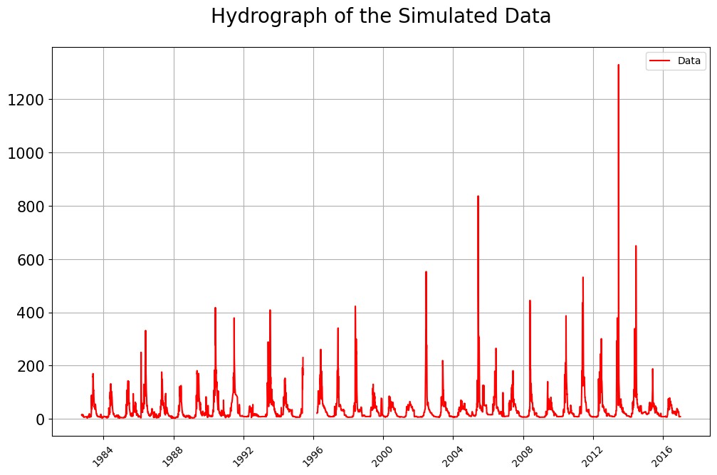
Starting off simple - one of the most important plots when working with hydrology and flow forecasting is the line plot of stream flow, stage or discharge. Using the data generated above we can plot these using our plot function. We are able to plot just single line data -
[4]:
# A very simple line plot can be generated as shown below
# Just plotting the simulated data from the first station
visuals.plot(
    df = DATAFRAMES["DF_OBSERVED"].iloc[:, [0]],
    title='Hydrograph of the Simulated Data',
    grid=True,
)
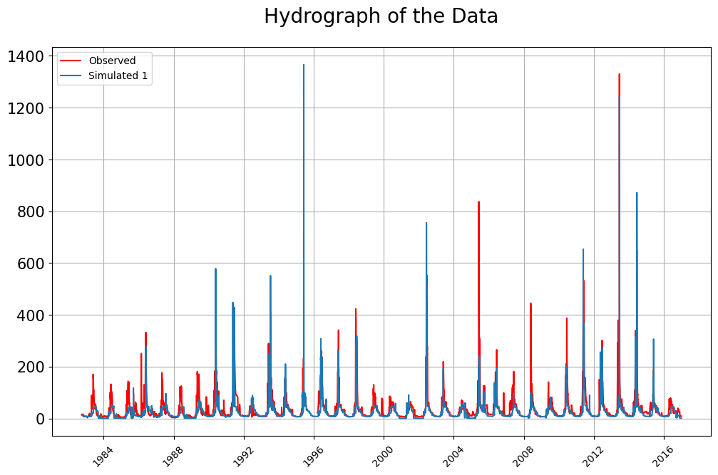
…and combined observed and simulated data -
[5]:
# Plotting both Observed and Simulated combined
visuals.plot(
    merged_df = DATAFRAMES["DF_MERGED"].iloc[:, [0, 1, 2]],
    title='Hydrograph of the Data',
    grid=True,
)
Number of simulated data columns: 1
Number of linewidths provided is less than the number of columns. Number of columns : 2. Number of linewidths provided is:  1. Defaulting to 1.5
Number of linestyles provided is less than the number of columns. Number of columns : 2. Number of linestyles provided is:  1. Defaulting to solid lines (-)
Number of legends provided is less than the number of columns. Number of columns : 2. Number of legends provided is:  1. Applying Default legend names
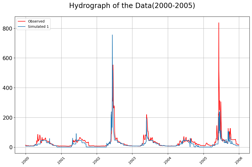
Lets zoom into a few years, say 2000-2005
[6]:
visuals.plot(
    merged_df = DATAFRAMES["DF_MERGED"]['2000-01-01':'2005-12-31'].iloc[:, [0, 1, 2]],
    title='Hydrograph of the Data(2000-2005)',
    grid=True,
)
Number of simulated data columns: 1
Number of linewidths provided is less than the number of columns. Number of columns : 2. Number of linewidths provided is:  1. Defaulting to 1.5
Number of linestyles provided is less than the number of columns. Number of columns : 2. Number of linestyles provided is:  1. Defaulting to solid lines (-)
Number of legends provided is less than the number of columns. Number of columns : 2. Number of legends provided is:  1. Applying Default legend names
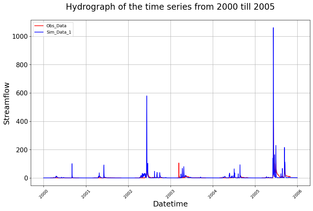
We are also able to plot just the simulated data in cases where we are not able to obtain them already merged together. This way we are not limited to a merged dataframe. Youd simply pass it in the way youd pass in merged. except you pass it into sim_df
The plot function also gives us complete control of the plot parameters. It allows you the flexibility to change the line colors, line width, axis labels, add grid lines, each plots title, the line legends and much more. There also exists an option to save the files as png images each with its own distinct name!
All the posibilities can be found over at the documentation website linked here. Some examples of these are shown below:
[7]:
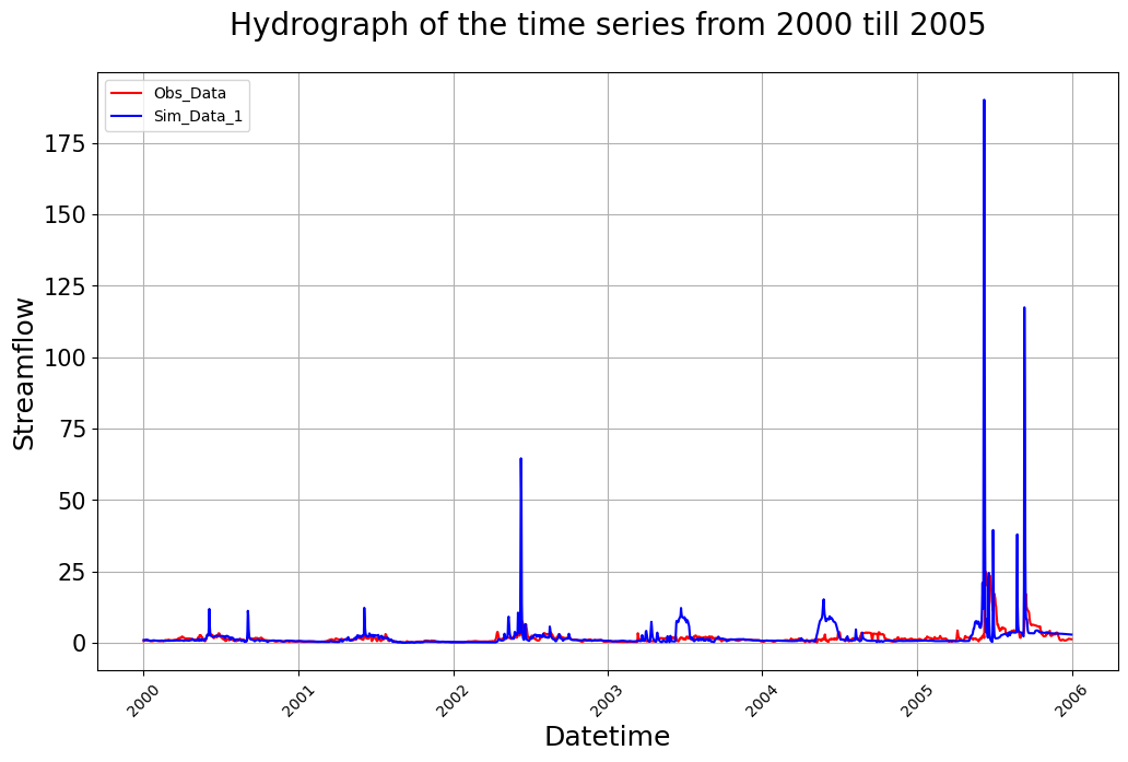
# Changing the default naming conventions
visuals.plot(
    merged_df =DATAFRAMES["DF_MERGED"]['2000-01-01':'2005-12-31'].iloc[:, [0, 1, 2, 3, 4, 5]],
    title='Hydrograph of the time series from 2000 till 2005',
    linestyles=('r-', 'b-', 'c-'),
    legend=('Obs_Data', 'Sim_Data_1','Sim_Data-2'),
    labels=('Datetime', 'Streamflow'),
    grid=True,
    )
Number of simulated data columns: 1
Number of linewidths provided is less than the number of columns. Number of columns : 2. Number of linewidths provided is:  1. Defaulting to 1.5

[8]:
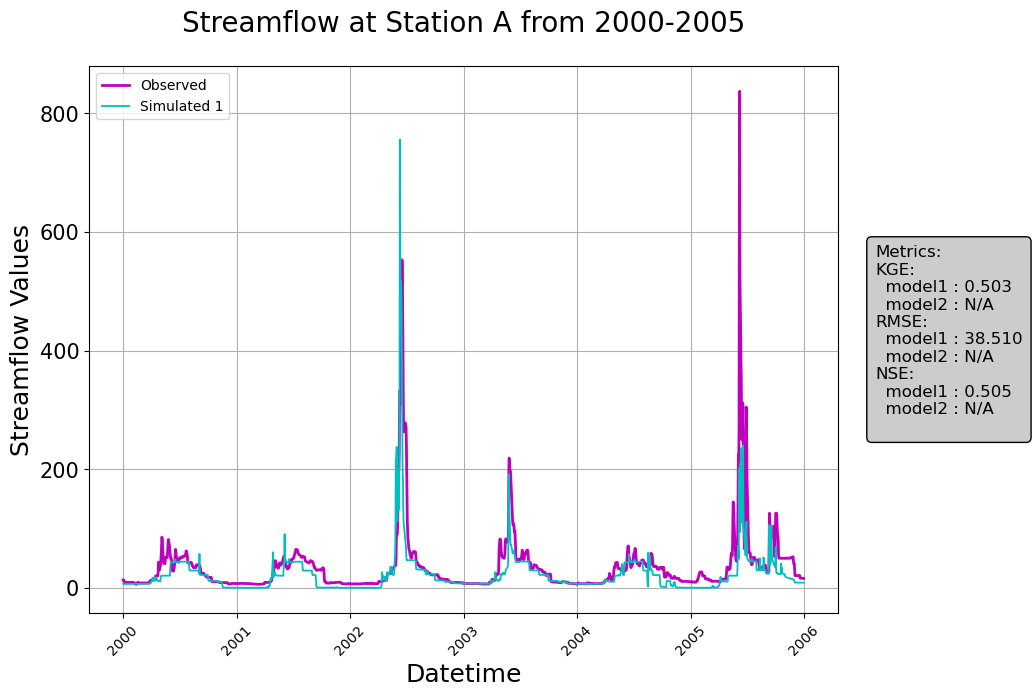
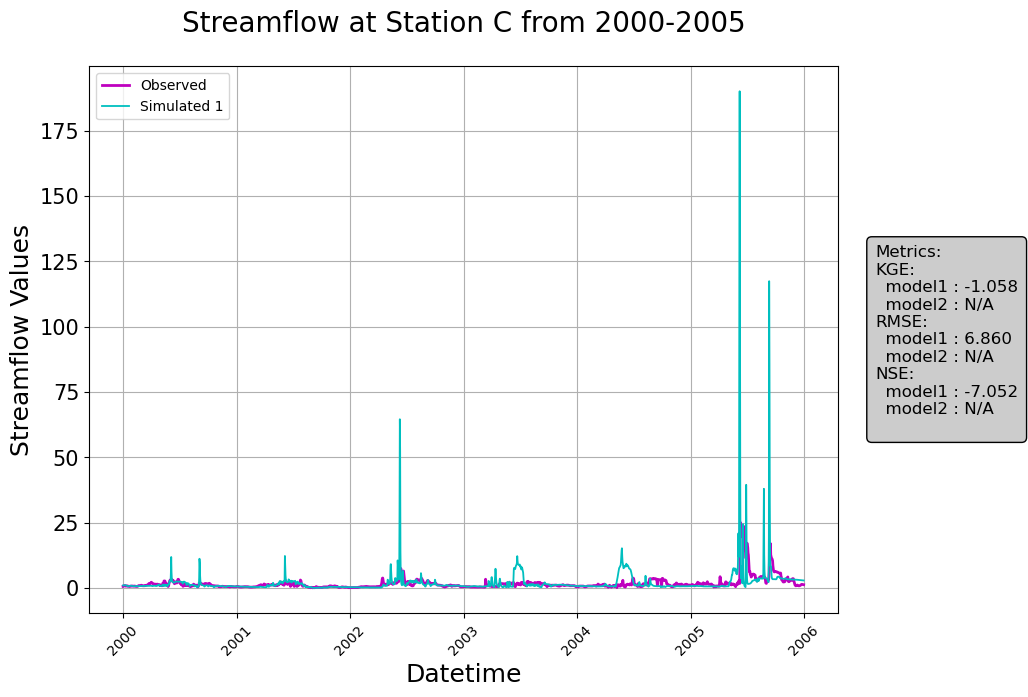
# Including the metrics in the plots for the 1st and 4th Stations
visuals.plot(
    merged_df =DATAFRAMES["DF_MERGED"]['2000-01-01':'2005-12-31'].iloc[:, [0, 1, 4, 5]],
    # including multiple plot titles
    title=['Streamflow at Station A from 2000-2005', 'Streamflow at Station C from 2000-2005'],
    fig_size=(10, 6),
    linestyles=['m-', 'c-'],
    labels=['Datetime', 'Streamflow Values'],
    linewidth=(2, 1.3),
    # include metrics
    metrices = ['KGE', 'RMSE', 'NSE'],
    grid=True,
    mode="models", models= ["model1", "model2"]
    # To save, uncomment the two lines below
    # save = True,
    # save_as = [station_a(2000-2005), station_b(2000-2005)],
    # The two images will be saved as png files with names as entered above in the current directory
    )
Number of simulated data columns: 1
Number of legends provided is less than the number of columns. Number of columns : 2. Number of legends provided is:  1. Applying Default legend names
BOUNDED PLOTS
Another really important plot is the bounded plot. The bounded plot is much like the line plot except it allows you to compare not just exact values but also the range of values. Within the MESH models evaluations, we use this when aggregating the data into days of the month, months of the year, etc. Its especially useful when trying to guage how accurate the range of values compared to say its median or mean for example. An exmaple is shown below
[9]:
visuals.bounded_plot(
    lines = DATAFRAMES["LONG_TERM_MEDIAN"].iloc[:, [0,1, 2, 3]],
    upper_bounds = [DATAFRAMES["LONG_TERM_MAX"].iloc[:, [0,1,2,3]]],
    lower_bounds = [DATAFRAMES["LONG_TERM_MIN"].iloc[:, [0,1,2,3]]],
    linestyles=['b-'],
    labels=['Datetime', 'Streamflow'],
    grid=True,
    transparency = [0.4, 0.3],
    title = 'Long term Median Aggregation compared to its max and min values'
    )
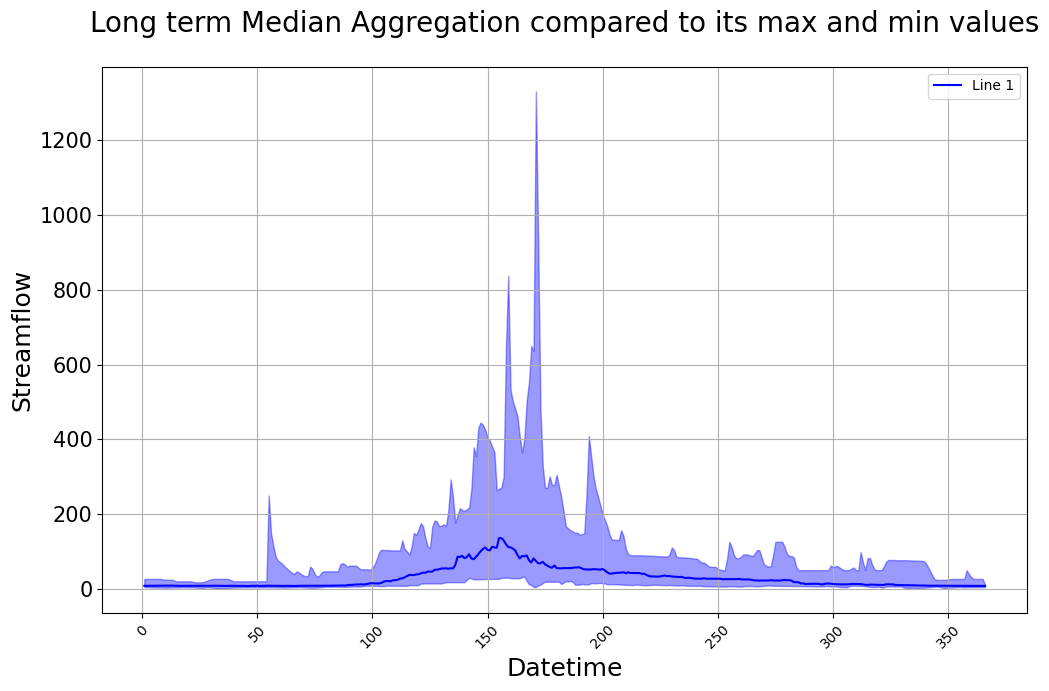
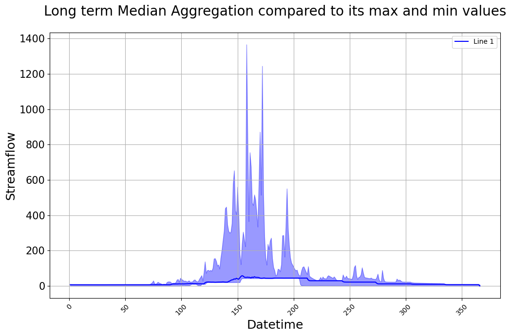
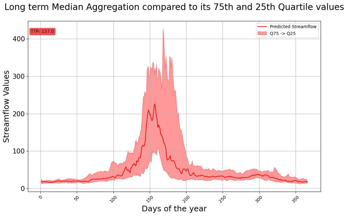
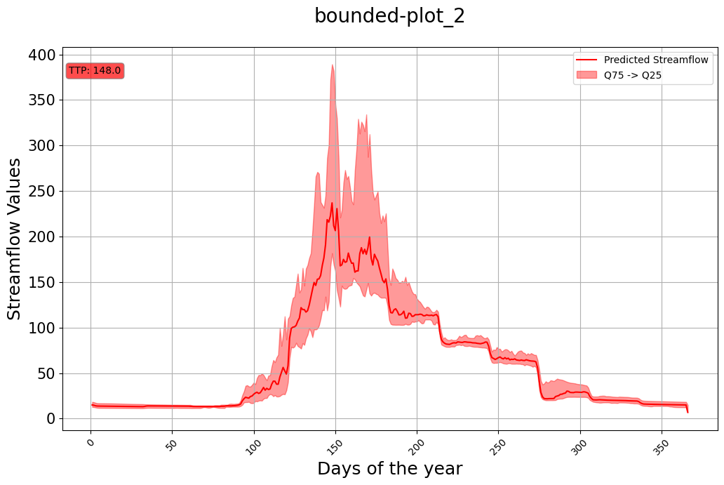
As you can see above, we compare the median of the long term aggregation to its max and min values. Below, lets compare it to the 25th and 75th Quartile values
[10]:
visuals.bounded_plot(
  lines = DATAFRAMES["LONG_TERM_MEDIAN"].iloc[:, [6,7]],
  upper_bounds = [DATAFRAMES["LONG_TERM_Q75"].iloc[:, [6,7]]],
  lower_bounds = [DATAFRAMES["LONG_TERM_Q25"].iloc[:, [6,7]]],
  title=['Long term Median Aggregation compared to its 75th and 25th Quartile values'],
  legend = ['Predicted Streamflow','Recorded Streamflow'],
  bound_legend = ["Q75 -> Q25"],
  linestyles=['r-'],
  labels=['Days of the year', 'Streamflow Values'],
    metrices=["TTP"],
  transparency = [0.4, 0.7],
  grid = 'True'
#   To save, uncomment the two lines below
#   save = True,
#   save_as = "b_plot_1", dir= '../b_plots'
)
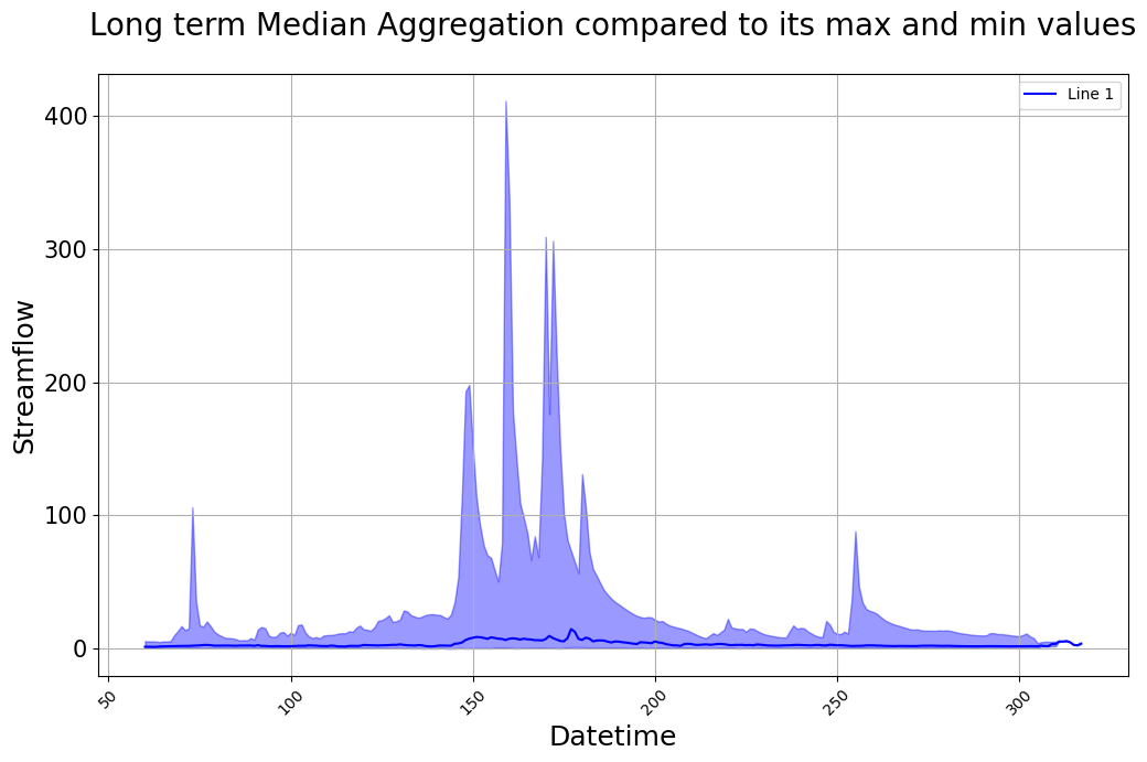
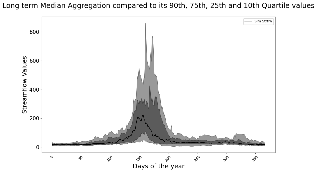
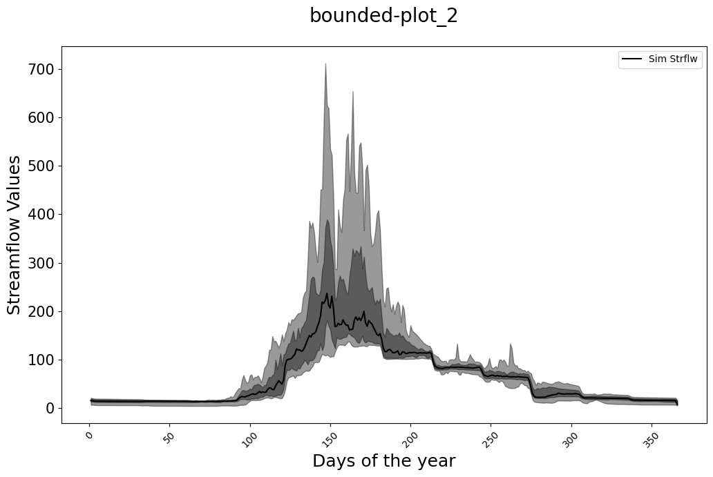
We can also use multiple bounds.
[11]:
visuals.bounded_plot(
  lines = DATAFRAMES["LONG_TERM_MEDIAN"].iloc[:, [6,7]],
  upper_bounds = [DATAFRAMES["LONG_TERM_Q75"].iloc[:, [6,7]], DATAFRAMES["LONG_TERM_Q90"].iloc[:, [6,7]]],
  lower_bounds = [DATAFRAMES["LONG_TERM_Q25"].iloc[:, [6,7]], DATAFRAMES["LONG_TERM_Q10"].iloc[:, [6,7]]],
  title=['Long term Median Aggregation compared to its 90th, 75th, 25th and 10th Quartile values'],
  legend = ['Sim Strflw','Obs Strflw'],
  linestyles=['k-', 'r-'],
  labels=['Days of the year', 'Streamflow Values'],
  transparency = [0.4, 0.25],
)
SCATTER PLOTS
The library provides us with two types of scatter plots. You select the one you want based on the inputs you pass into it.
The first kind directly compares simulated or predcicted data (i.e., data generated by using the models) to actual oberved or measure data. It is used to visually show how accurately the model predicts the data. The closer the points are to the 45 degree line the more accurate the model is. Its is also used to show areas and time periods where the data does better which might point to a different problem such as weather anomalies, instrument errors, etc.
An example is shown below
[12]:
visuals.scatter(merged_df = DATAFRAMES['DF_MERGED']['1981-01-01':'1985-01-31'].iloc[:, [4, 5]],
               grid = True,
               labels = ("Simulated Data", "Observed Data"),
               markerstyle = ['r.'],
               title = "Scatterplot of the data from January 1981 to January 1985",
               line45 = True,
               metrices = ['KGE', 'RMSE'],
#                save = True,
               )
Number of simulated data columns: 1
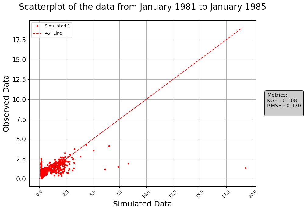
Similar to the other plots, there’s ways to save the images using the save, save as and dir parameters passed into the function. It also allows the calculations of metrics as shown above.
Another way to use the function would be using to show variations in certain metrics to show where the models performs better for that particular metric. You will have to provide some sort of shapefile and the parameters you’d need to plot it like x and y axis values, and the metric you’d be comparing.
An example is shown below:
[13]:
shapefile_path = r"SaskRB_SubDrainage2.shp"

visuals.scatter(shapefile_path = shapefile_path,
    title = "SRB SubDrainage showing the NSE distribution",
    x_axis = Stations["Lon"],
    y_axis = Stations["Lat"],
    metric = "NSE",
    fig_size = (24, 30),
    observed = DATAFRAMES["DF_OBSERVED"],
    simulated = DATAFRAMES["DF_SIMULATED"],
    labels=['Longitude', 'Latitude'],
#     mode = "models",
#     models = ["model1"],
#     cmap = 'viridis',
#     vmin = 0,
#     vmax=0.8,
)
C:\Users\udenzeU\Desktop\JUPYTER\postprocessing\docs\source\notebooks\../../..\postprocessinglib\evaluation\visuals.py:187: UserWarning: This figure includes Axes that are not compatible with tight_layout, so results might be incorrect.
  plt.tight_layout()
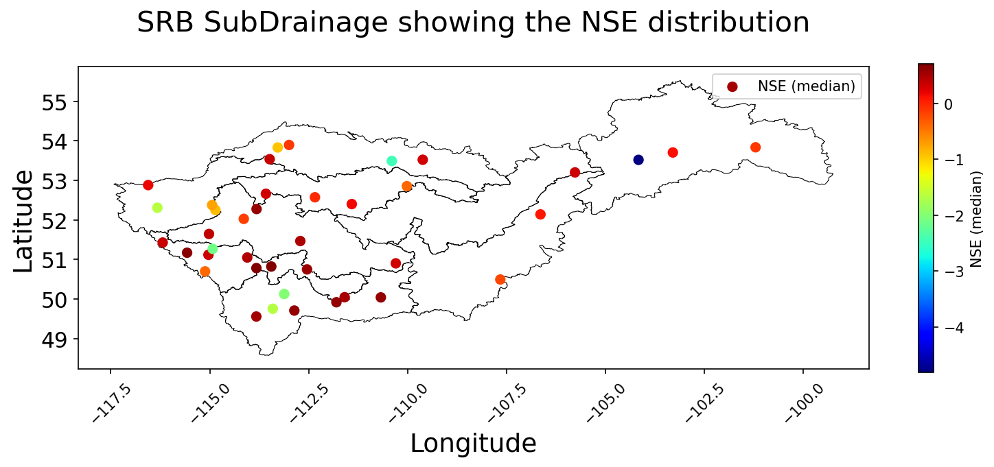
The graph above shows the location of various stations and how accurately the models predict the streamflow by using the KGE (Kling - Gupta Efficiency) metric. You are also allowed to change the color scheme of your cmap, the maximum and minimum values of your color map and just like the ones above, you can also save using the respective parameters like the above visualizations tools.
HISTOGRAM PLOTS
The histogram compares the distribution of observed and simulated data, providing insights into their statistical characteristics and variability. Its allows users to analyze the frequency distribution of hydrological data, assess model performance, and identify biases in the simulated dataset.
its features are very similar to that of the line plot where we are able to plot single data using the df argument and plot observed and simulated data. Some of these functionality is shown below
[14]:
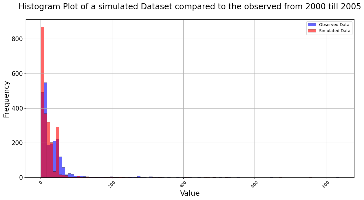
visuals.histogram(
    merged_df =DATAFRAMES["DF_MERGED"]['2000-01-01':'2005-12-31'].iloc[:, [0, 1]],
    grid = True,
    title = "Histogram Plot of a simulated Dataset compared to the observed from 2000 till 2005",
)
[15]:
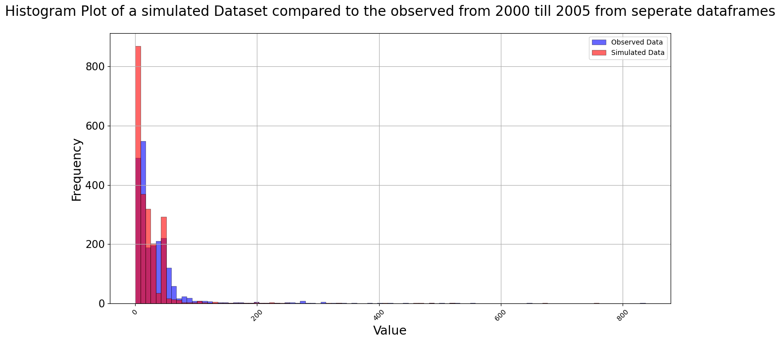
visuals.histogram(
    obs_df =DATAFRAMES["DF_OBSERVED"]['2000-01-01':'2005-12-31'].iloc[:, [0]],
    sim_df =DATAFRAMES["DF_SIMULATED"]['2000-01-01':'2005-12-31'].iloc[:, [0]],
    grid = True,
    title = "Histogram Plot of a simulated Dataset compared to the observed from 2000 till 2005 from seperate dataframes",
)
[16]:
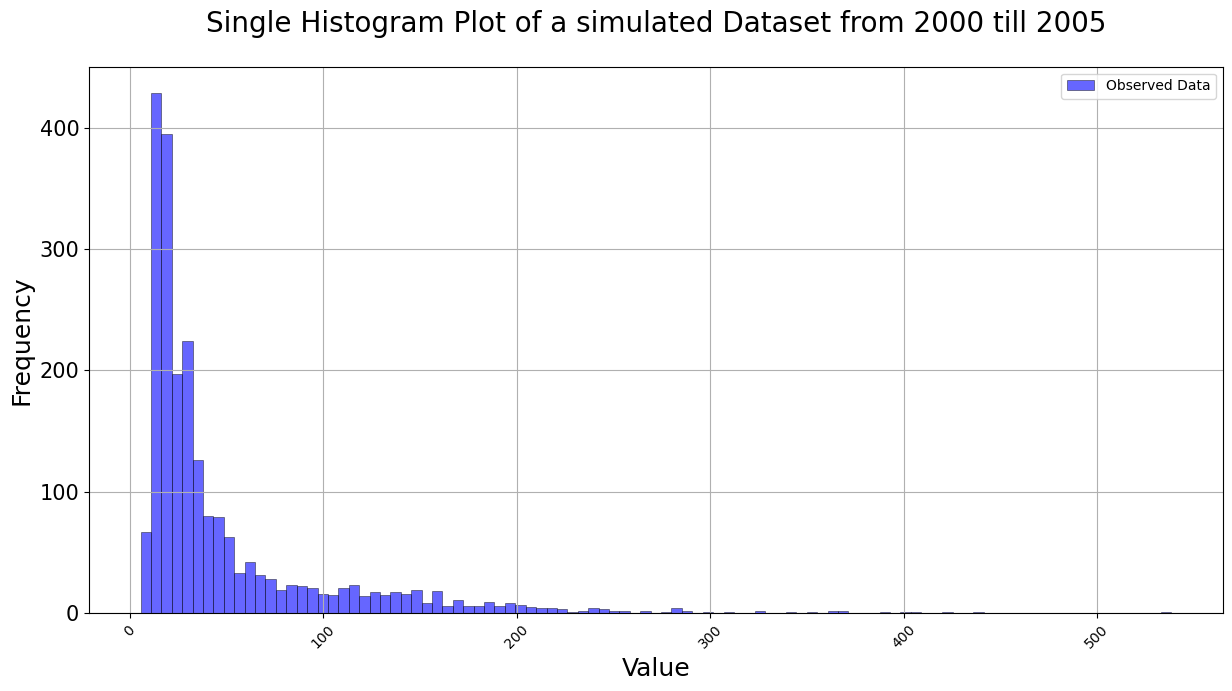
visuals.histogram(
    df =DATAFRAMES["DF_SIMULATED"]['2000-01-01':'2005-12-31'].iloc[:, [8]],
    grid = True,
    title = "Single Histogram Plot of a simulated Dataset from 2000 till 2005",
)
You are able to modify the numbers of bins/bars, you are able to specify if you want the data z-normalized as well as specify if you want the data normalized to form a probability density as shown below:
[17]:
visuals.histogram(
    df =DATAFRAMES["DF_SIMULATED"]['2000-01-01':'2005-12-31'].iloc[:, [8]],
    grid = True,
    title = "Histogram Plot of the simulated Dataset from 2000 till 2005",
    prob_dens = True, bins = 75,
    colors = ['', 'g']
)
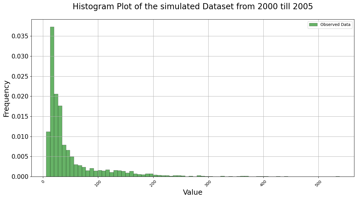
By setting the probability density to true, the plot gets normalized to a state where the area under the graph equals to 1. i.e the area of each bar summed up will equal 1.
[18]:
visuals.histogram(
    df =DATAFRAMES["DF_SIMULATED"]['2000-01-01':'2005-12-31'].iloc[:, [8]],
    grid = True,
    title = "Histogram Plot of the simulated Dataset from 2000 till 2005",
    z_norm = True, bins = 75,
    colors = ['', 'g']
)
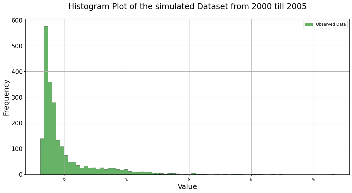
As observed, the data has been z score normalized.
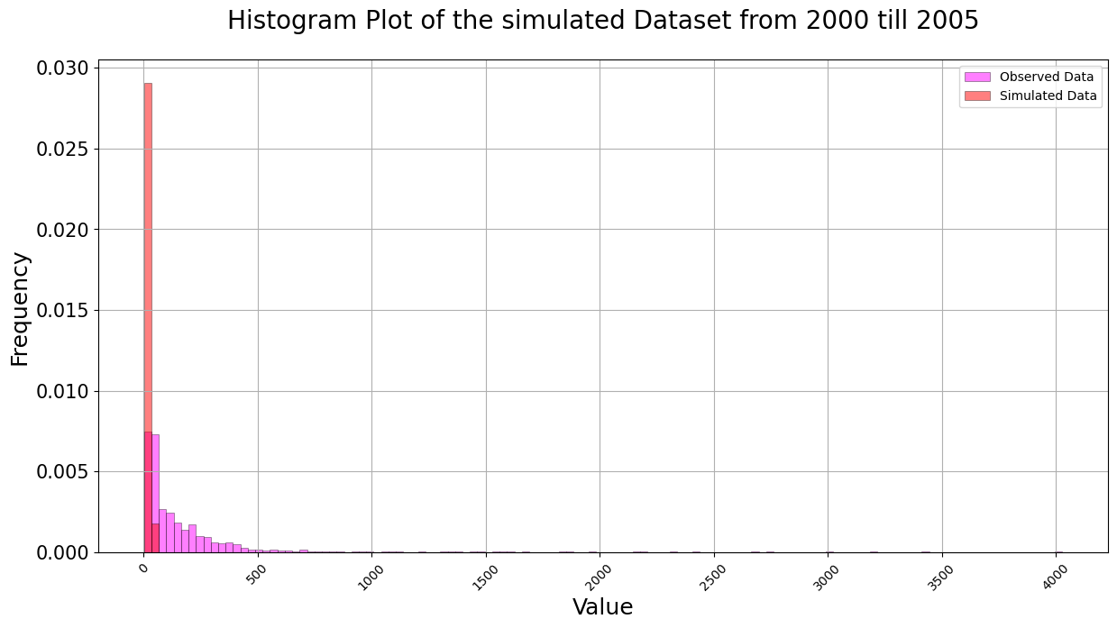
As usual you are also able to modify the color, transparency of the bars and size of the figure, amongst others. You are also able to save the figures
[19]:
visuals.histogram(
    merged_df =DATAFRAMES["DF_MERGED"]['2000-01-01':'2005-12-31'].iloc[:, [9, 10]],
    grid = True,
    title = "Histogram Plot of the simulated Dataset from 2000 till 2005",
    prob_dens = True, bins = 125,
    colors = ['red', 'magenta'],
    transparency = 0.5,
#     save=True,
#     save_as="histogramplot_example",
#     dir = '../Figures'
)
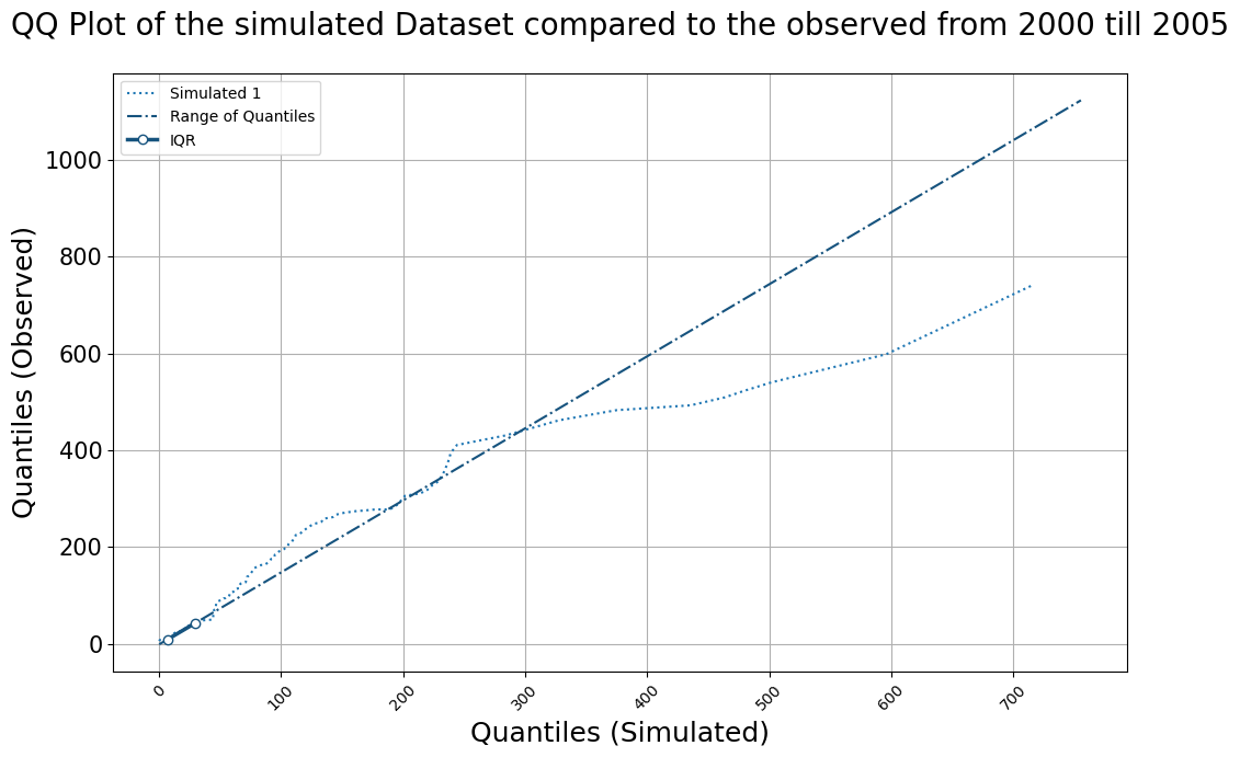
QUANTILE QUANTILE PLOTS
The Quantile plot allow us to immediately see if the observed and simulated datsets - when plotted against each other - follow the normal distribution by comparing their quantiles i.e., we compare the quantiles of the simulated dataset to that of the observed and see how accurately they fall on the y = x line.
[20]:
visuals.qqplot(
    merged_df =DATAFRAMES["DF_MERGED"]['2000-01-01':'2005-12-31'].iloc[:, [0, 1]],
    labels=["Quantiles (Simulated)", "Quantiles (Observed)"],
    title="QQ Plot of the simulated Dataset compared to the observed from 2000 till 2005",
    grid = True
)
Number of simulated data columns: 1
Our library also allows us to plot a quantile range within which certain qauntiles will exist. Its default is the interquartile range of the 25th to the 75th Quartile but you are able to adjust it to whatever you want and name it how ever you want. For example:
[21]:
visuals.qqplot(
    merged_df =DATAFRAMES["DF_MERGED"]['2000-01-01':'2005-12-31'].iloc[:, [16, 17]],
    labels=["Quantiles (Simulated)", "Quantiles (Observed)"],
    title="QQ Plot of the simulated Dataset comapred to the observed from 2000 till 2005",
#     legend = True,
    quantile = [75, 100],
    q_labels= ['','','Upper Quantile'],
    grid = True
)
Number of simulated data columns: 1
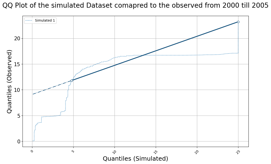
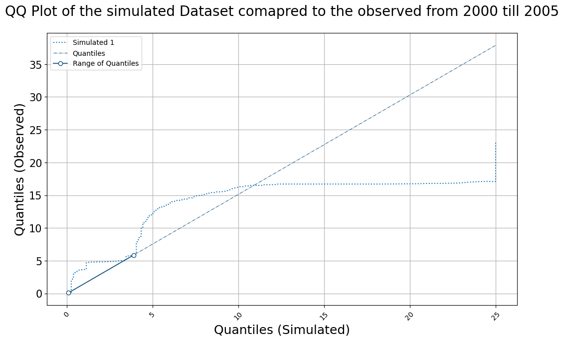
As usual you able to modify the shape, color and thickness of your lines as you see fit and you are able to save the images as well as shown in previous plots
[22]:
visuals.qqplot(
    merged_df =DATAFRAMES["DF_MERGED"]['2000-01-01':'2005-12-31'].iloc[:, [16, 17]],
    linestyle = ['r:','c-.','k-'],
    labels=["Quantiles (Simulated)", "Quantiles (Observed)"],
    title="QQ Plot of the simulated Dataset comapred to the observed from 2000 till 2005",
    linewidth = [.75, 1.25],
#     legend = True,
    quantile = [0, 50],
    q_labels= ['Quantiles','Range of Quantiles','Lower Half'],
    grid = True,
#     save=True,
#     save_as="qqplot_example",
#     dir = '../Figures'
)
Number of simulated data columns: 1
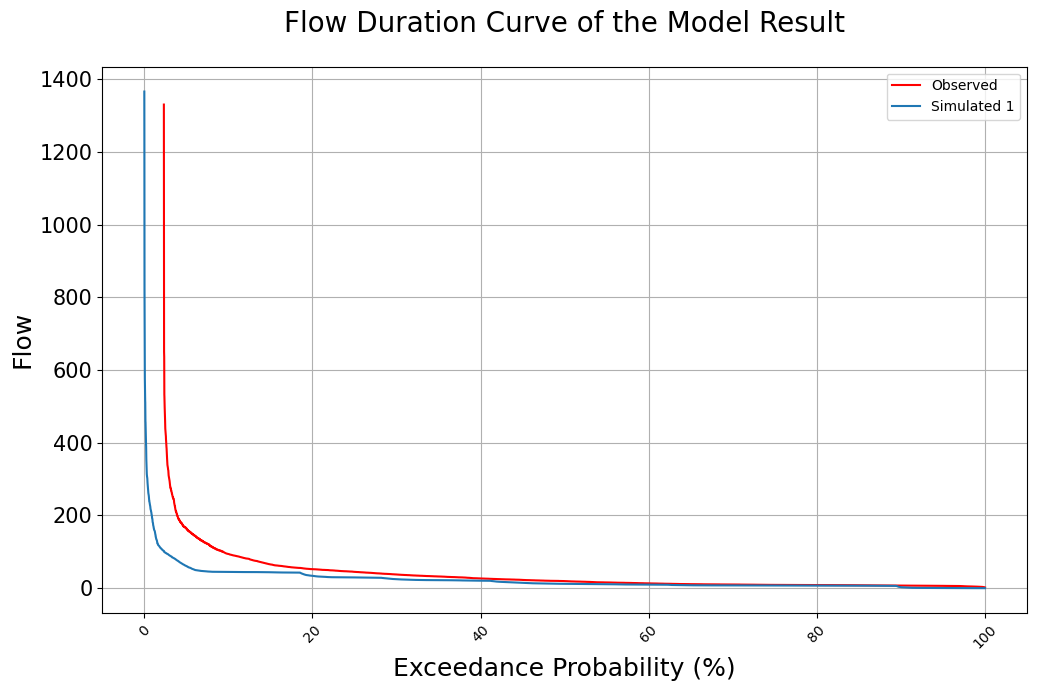
FLOW DURATION CURVE
The Flow Duration Curve (FDC) is a graphical representation of the frequency distribution of flow values, showing the relationship between exceedance probability and streamflow magnitude. This function compares the observed and simulated data sets and generates the FDC for each column in the provided data. This is shown below:
[23]:
visuals.flow_duration_curve(
    merged_df = DATAFRAMES["DF_MERGED"].iloc[:, [0, 1]],
    title='Flow Duration Curve of the Model Result',
    grid = True
)
Number of simulated data columns: 1
Number of linewidths provided is less than the number of columns. Number of columns : 2. Number of linewidths provided is:  1. Defaulting to 1.5
Number of linestyles provided is less than the number of columns. Number of columns : 2. Number of linestyles provided is:  1. Defaulting to solid lines (-)
Number of legends provided is less than the number of columns. Number of columns : 2. Number of legends provided is:  1. Applying Default legend names
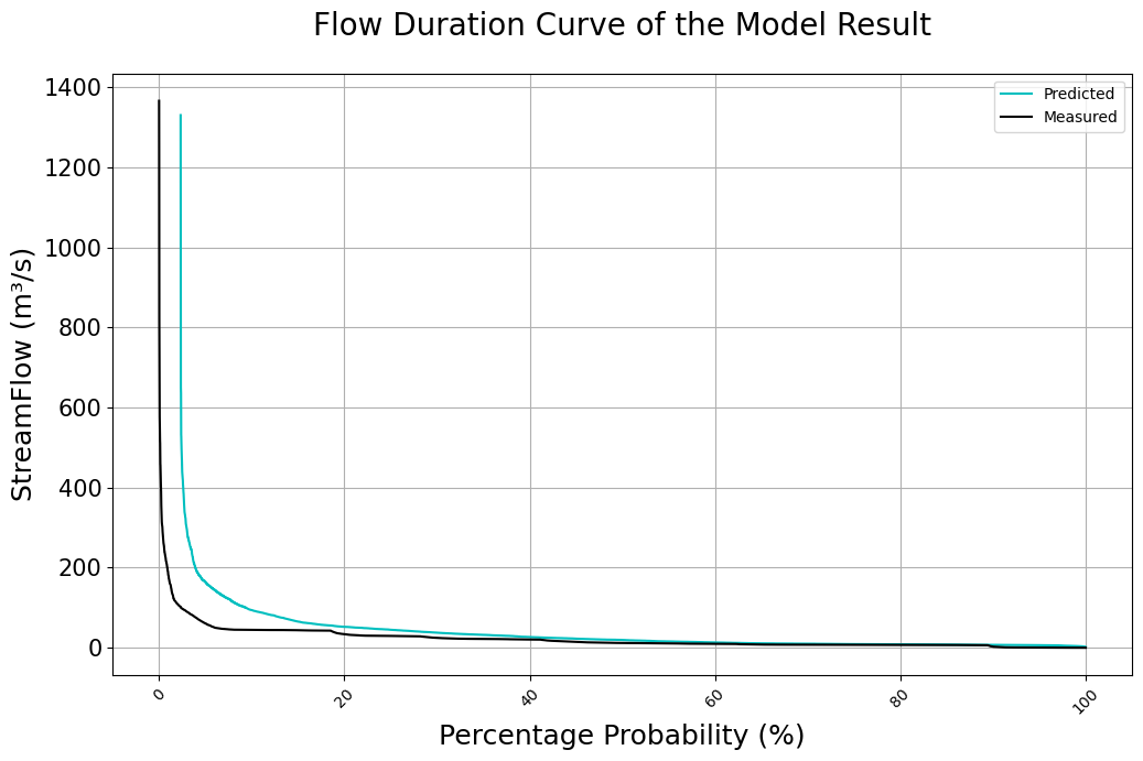
As usual you are able to modify the plot parameters as you see fit - everything from colors to names to labels names and plot size - and of course, you can save the images generated
[24]:
visuals.flow_duration_curve(
    merged_df = DATAFRAMES["DF_MERGED"].iloc[:, [0, 1]],
    title='Flow Duration Curve of the Model Result',
    legend=['Predicted','Measured'],
    labels=('Percentage Probability (%)', 'StreamFlow (m³/s)'),
    linestyles=('c-', 'k-'),
    grid = True,
#     save=True,
#     save_as="FDC_example",
#     dir = '../Figures'
)
Number of simulated data columns: 1
Number of linewidths provided is less than the number of columns. Number of columns : 2. Number of linewidths provided is:  1. Defaulting to 1.5
[ ]:
[ ]: